
Illya Starikov
Last week I traveled back to my parents. After a rewarding yet exhausting month at work, travel, and COVID, I felt it was time to reconnect with nature.
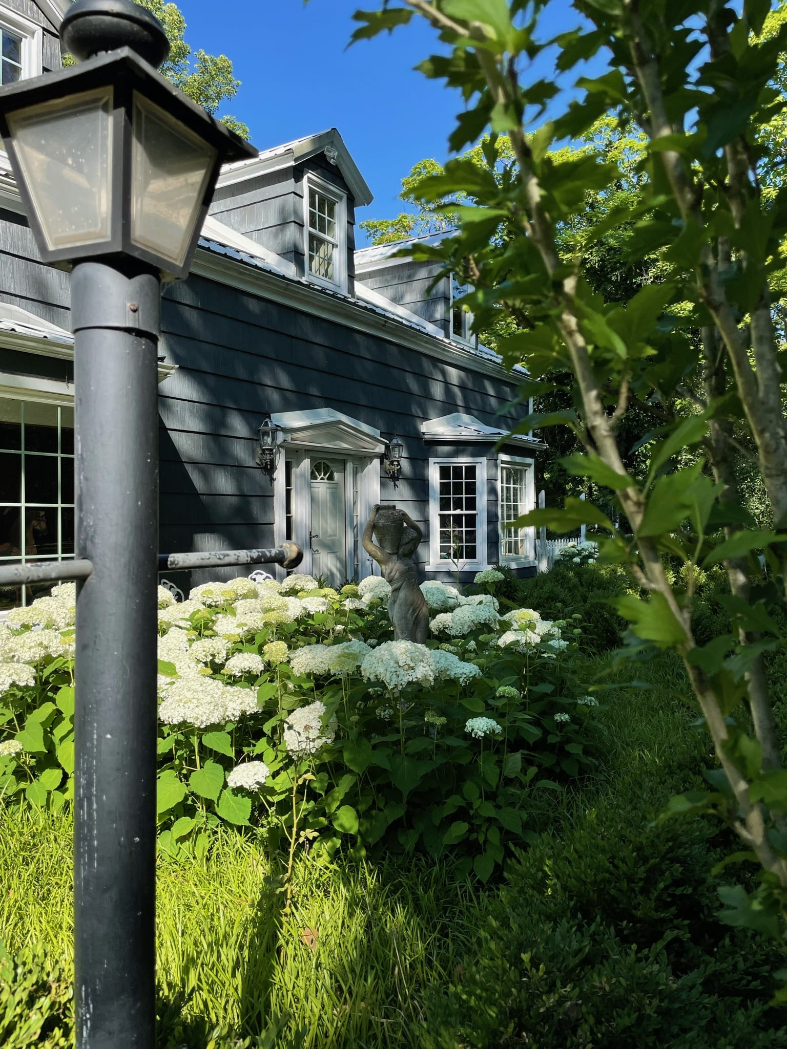
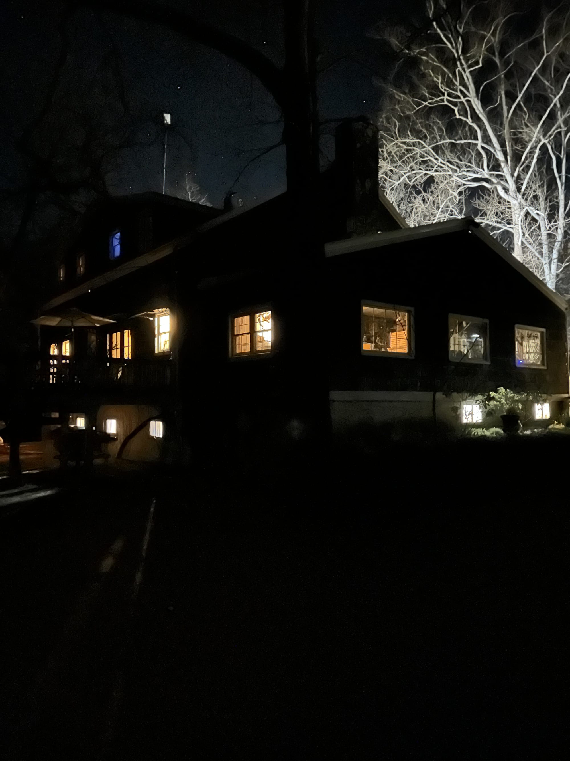
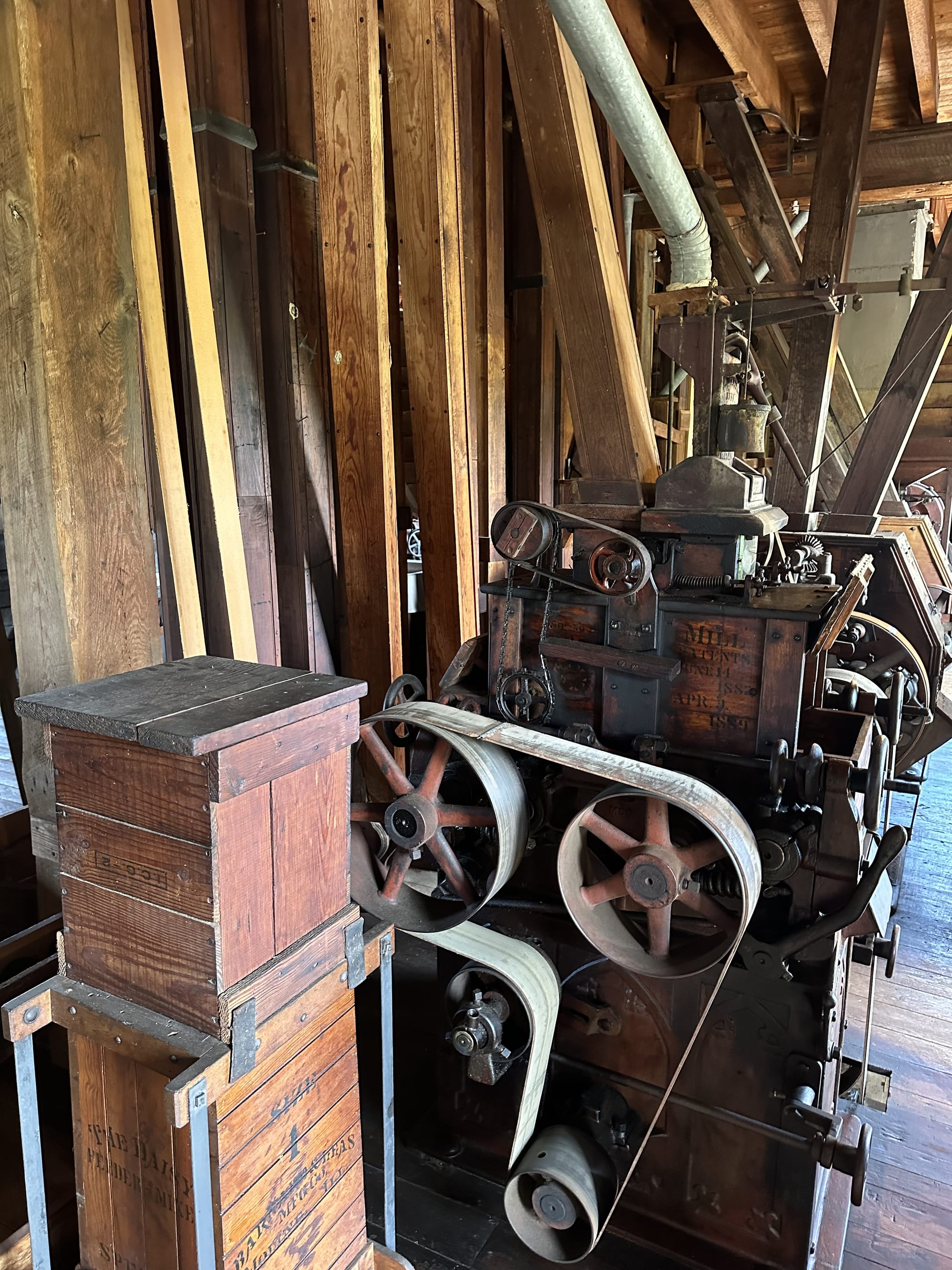
My mom and I moved to Missouri in April of 2001, where I would remain until I graduated high school. The house has belong to my dad’s family for over 40 years now, it bears a lot of memories in its wooden bones.
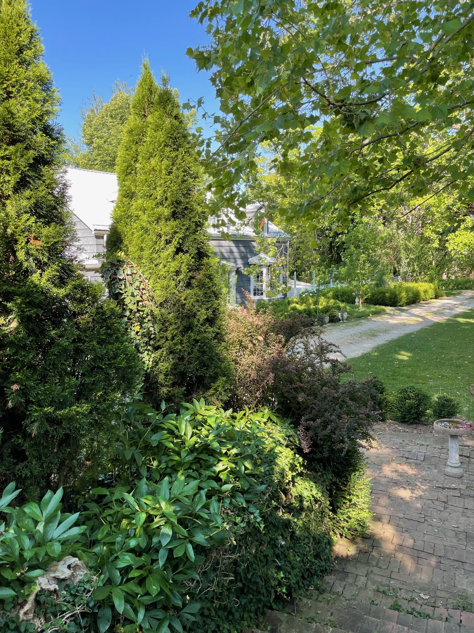
The house is as rural as they come: the closest neighbor is a mile away and the closest town fifteen, everyone asks how you are even if they don’t know you, sometimes cows escape and you have to corral them back to Donna’s house. It’s quant and rustic, traditional, slow-paced and remote. A place for me to be one with the trees.


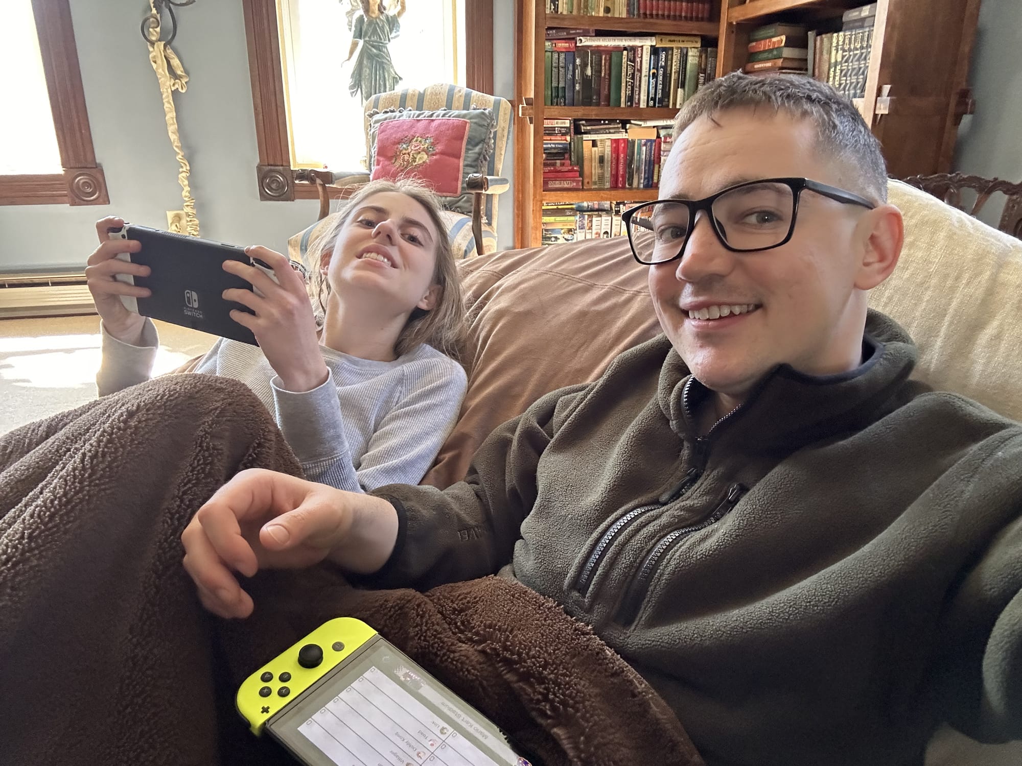
During my stay I got lots of family time. My mom’s favorite past time is going for a walk down to the river. Dad and I have more of a TV dynamic, and we mean business. In the five days of consumption we managed to watch two 2hr movies and ten episodes of friends — regularly finishing up around 1am. My sister and I do the same thing we’ve been doing since she was young: video games, namely, Mario Kart and Smash Bros.
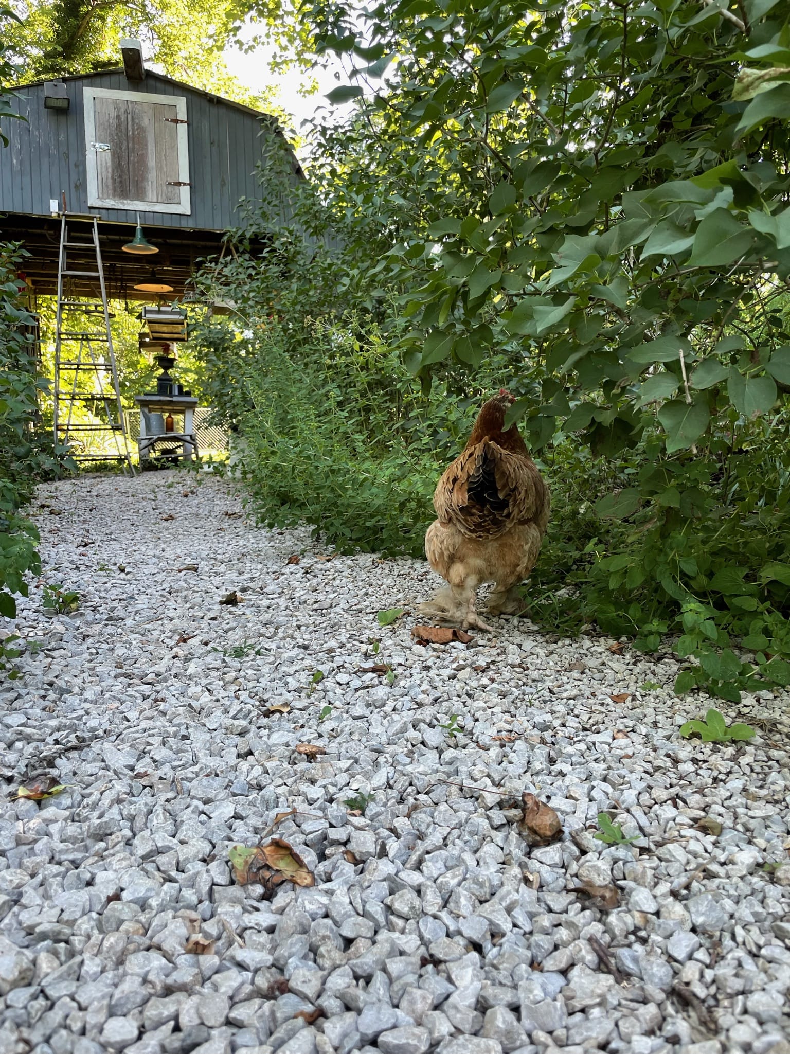
Along with my parents, there’s a lovely dog Marley and Satan-disguised-as-a-bird George.
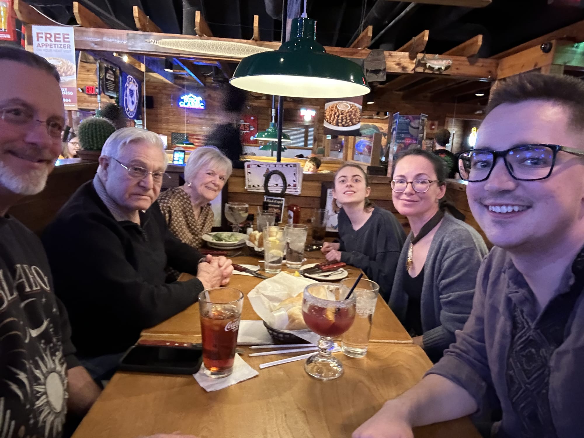
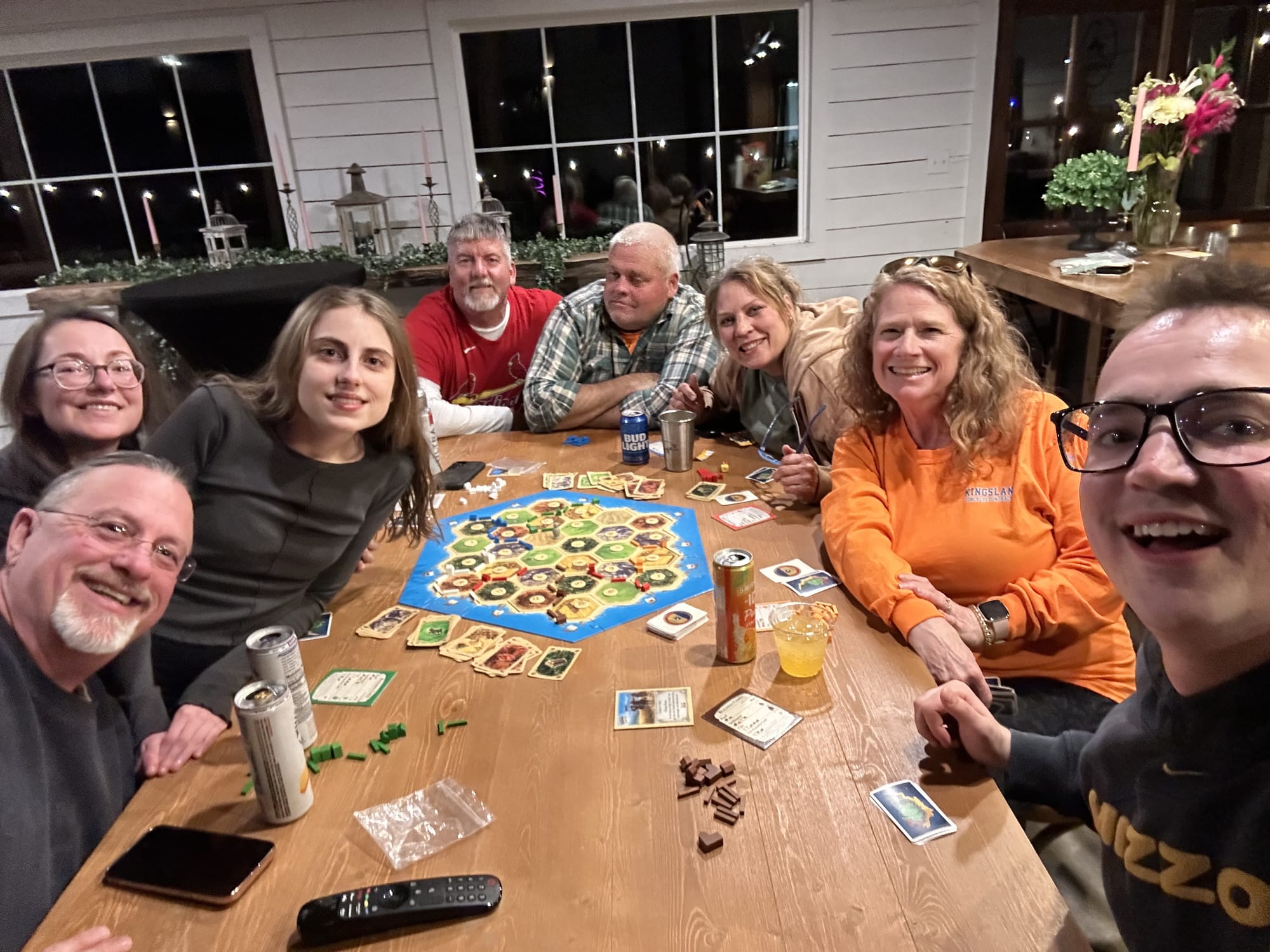
When I wasn’t home with my parents, we were visiting extended family. A friend of the family Kim put up a barn with a disco ball. We played board games — and I played Settlers of Catan for the first time! We had our ceremonial steak dinner at Texas Roadhouse. Steak — and meat in general — is a staple of our home. So much so, we had it for five meals.
Along with steaks, my mom took time to make some Ukrainian staples: borscht and holubsi. I only have photos of mom making them. By the time everything was finished cooking I had a singular focus: food in my belly.


Besides family time, we were able to see some really iconic sites.
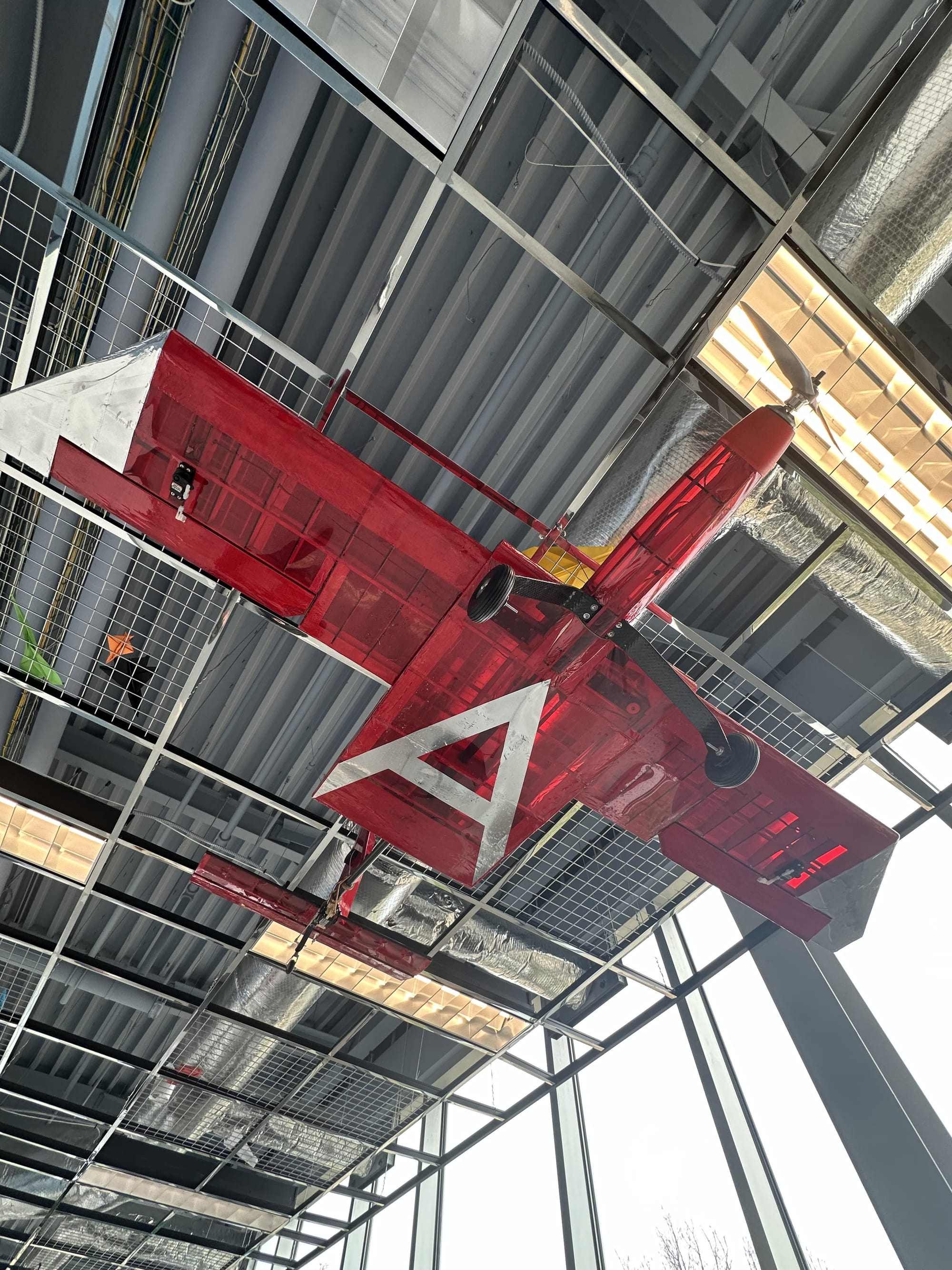
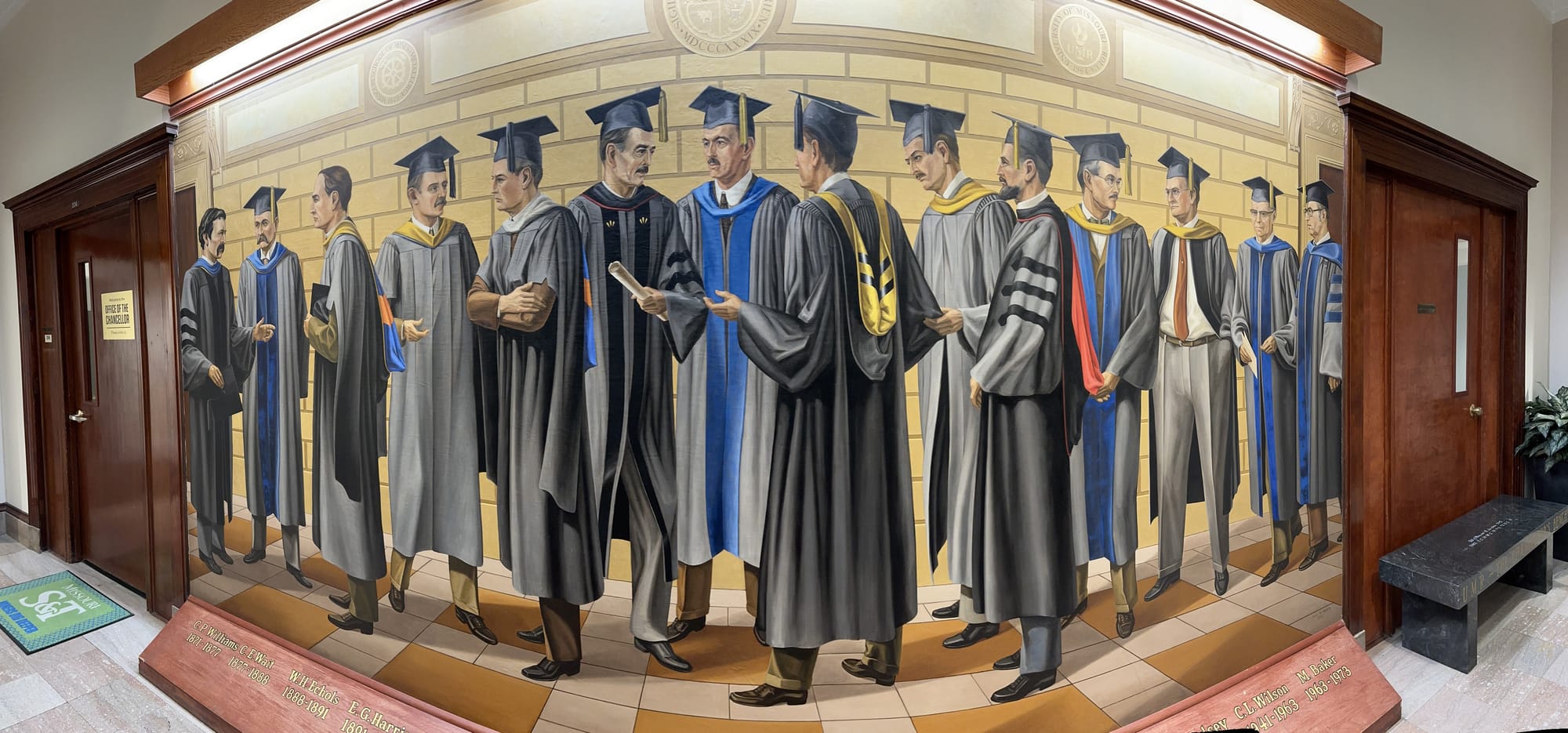
We got to see my Alma Mater Missouri S&T. I was proud to show my parents the same buildings I spent four years in. Toomey Hall, where I was part of the S&T Satellite Team, who recently launched a satellite into space! The library, where I spent so much time that I found the optimal nap spots. The computer science building, which finally got an expansion it so desperately needed. I also got to see my grandma’s house near the college; it felt like a genuine legacy moment.


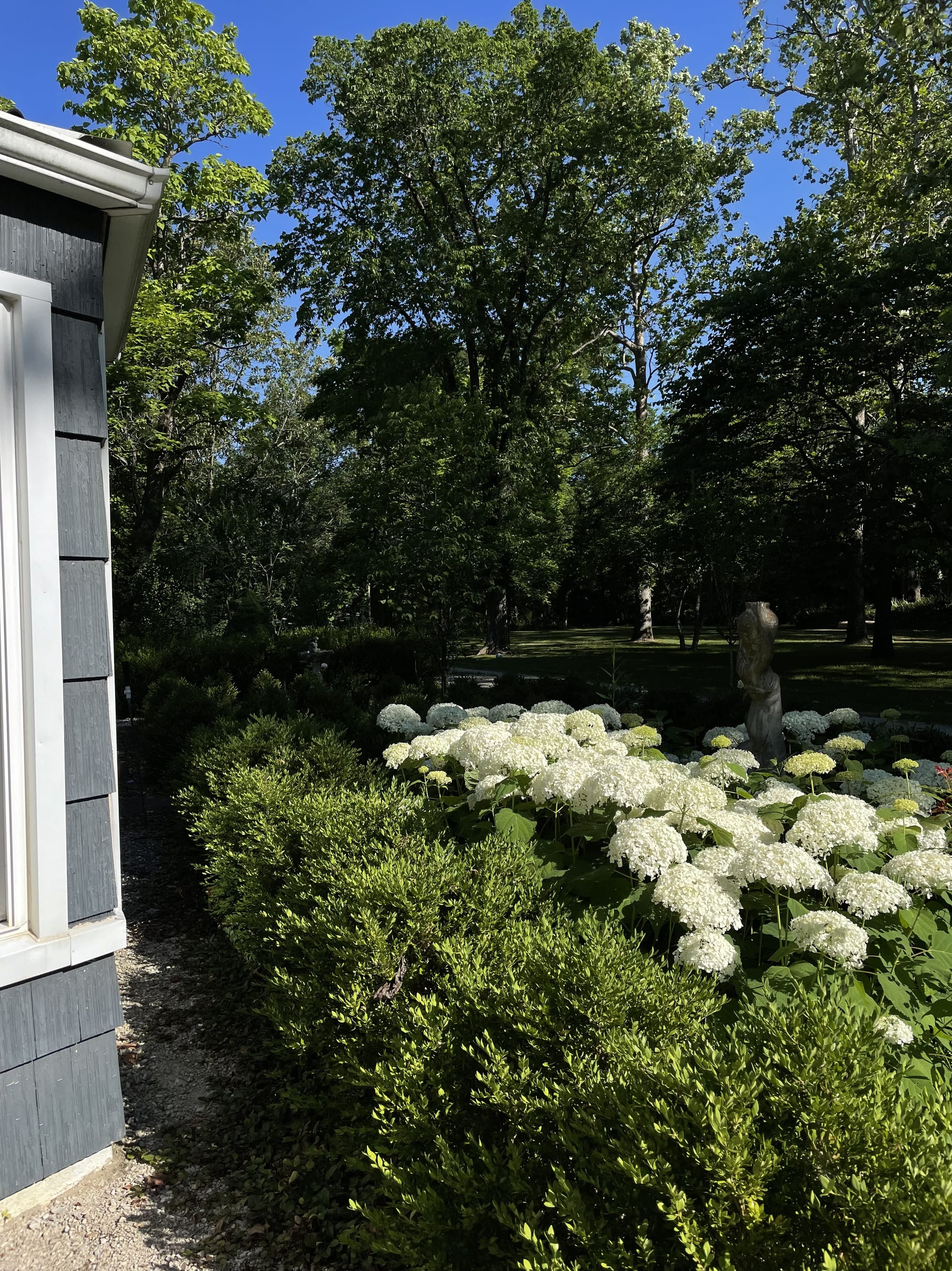
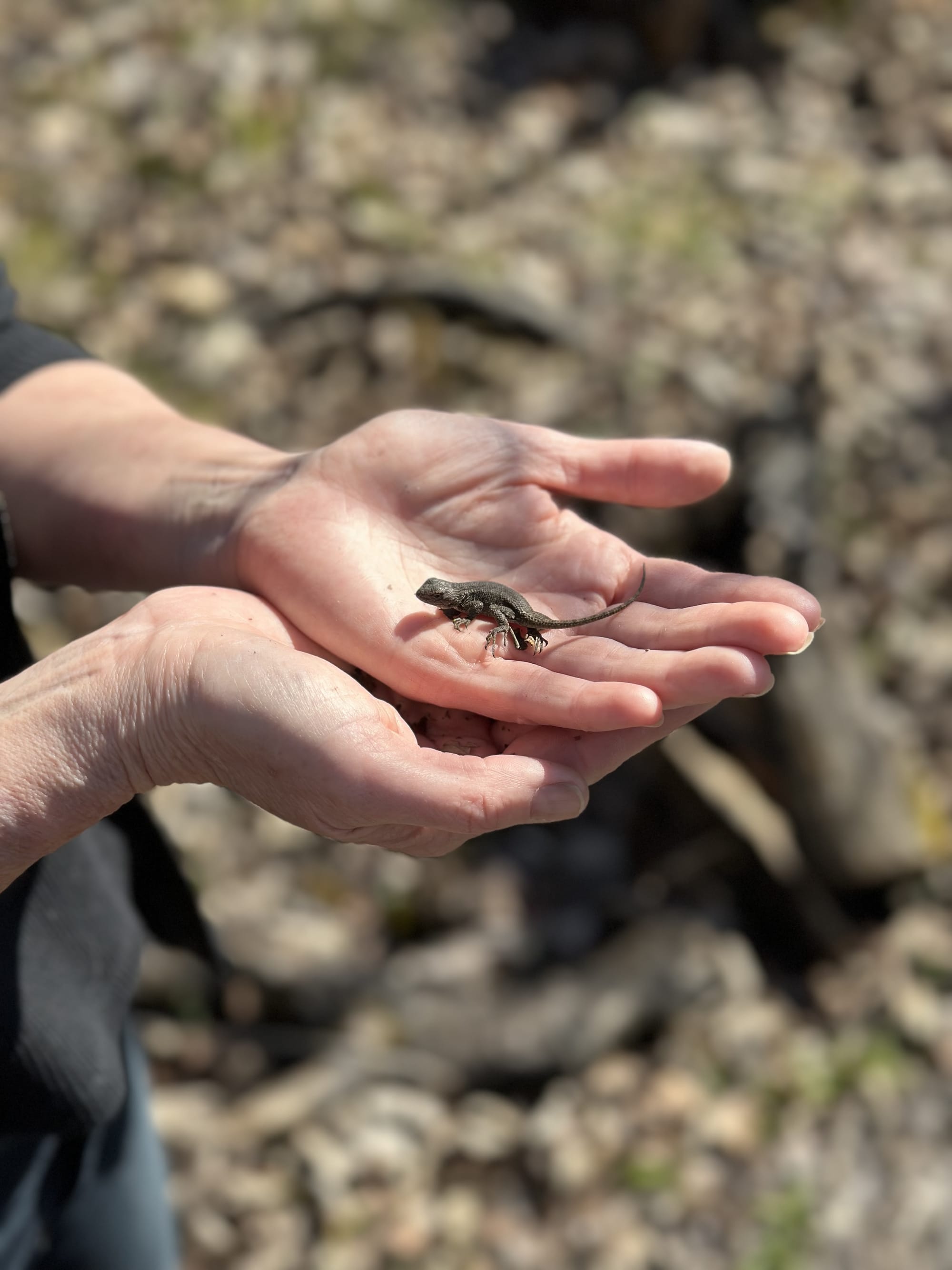
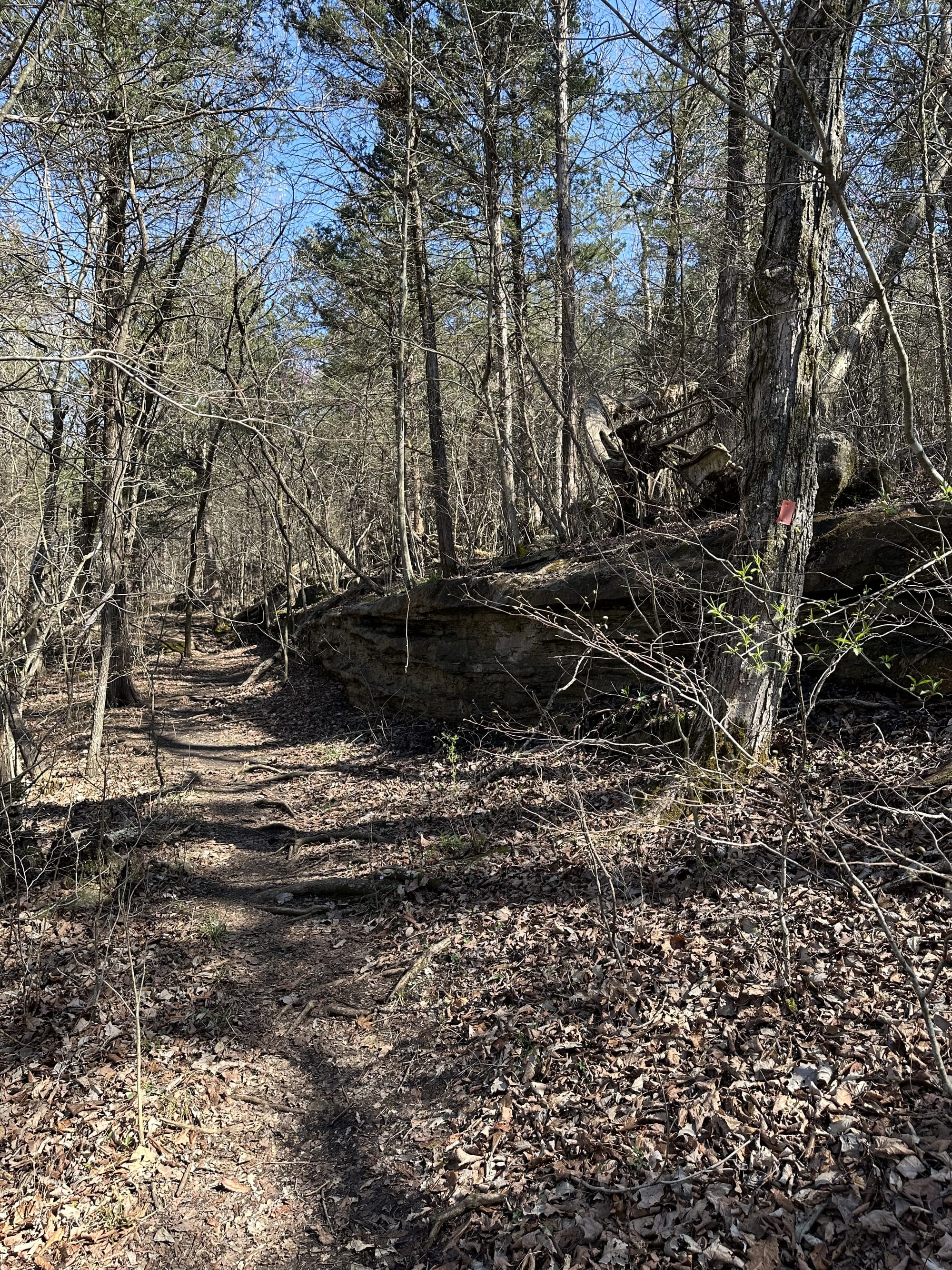
It wouldn’t be home if I didn’t talk about the nature. Although we have a state park a mere five minutes away, the nature is plentiful right outside the door. Going on a walk you might see something new every day.


Now, I returned to the Bay Area. Refreshed, recharged, ready to tackle new problems in new ways. Until next time, Mom and Dad.
Bookmarked Books 📚
So many books, so little time.
The following are my favorite books I’ve read. I’ve added them here in the hopes you might like some of them too. For a full list, check out my Goodreads.
Fiction
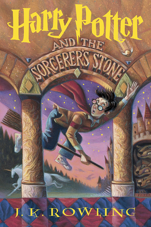

- The Harry Potter series 1 2 3 4 5 6 7
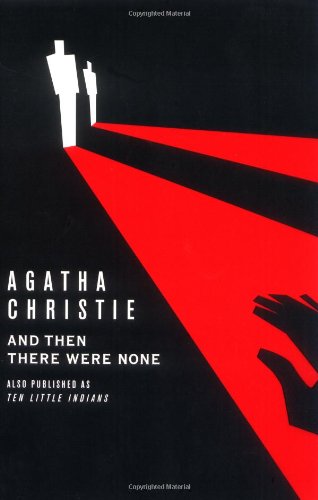
- And Then There Were None
- The Great Gatsby
- Treasure Island
Non-Fiction


- Red Famine: Stalin's War on Ukraine
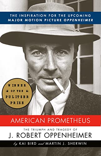
- American Prometheus
- Getting Things Done: The Art of Stress-Free Productivity
- I'm Glad My Mom Died
- Kitchen Confidential: Adventures in the Culinary Underbelly
- The Antidote: Happiness for People Who Can't Stand Positive Thinking
- The Gates of Europe: A History of Ukraine
- Masters of Doom: How Two Guys Created an Empire and Transformed Pop Culture
- The Hidden Brain: How Our Unconscious Minds Elect Presidents, Control Markets, Wage Wars, and Save Our Lives
- Hold Me Tight: Seven Conversations for a Lifetime of Love
- How Google Works
- The Theory of Poker: A Professional Poker Player Teaches You How To Think Like One
Textbooks
- New Year’s Day Новий Рік January 1
- Unity Day January 16
- Cyborg Remembrance Day January 20
- Mourning Day of the Beginning of the Russian invasion of Ukraine February 24
- International Women’s Day Міжнародний жіночий день March 8
- Labour Day День праці May 1
- Easter
- Second World War Remembrance Day May 7
- Victory Day (over Nazism in World War II) День пам'яті та перемоги над нацизмом у Другій світовій війні May 8
- Trinity (Pentecost) Трійця
- Constitution Day День Конституції України June 28
- Statehood Day День Української Державності July 15
- Flag Day August 23
- Independence Day of Ukraine День Незалежності України August 24
- Day of Knowledge September 1
- Ukraine Defender Day День захисників і захисниць України October 1
- Teacher’s Day October 2
- Holodomor Memorial Day Final Saturday of November
- Armed Forces of Ukraine Day December 6
- Christmas Різдво Христове December 25
The following are films about the 2014 invasion-present day war. Viewer discretion advised.
Directly from Ukraine
- ETNODIM
- Aviatsiya Halychyny
- Shkoura
- Sleeper (women only)
- O.TAJE (women only)
Support Ukraine directly
Non-Fiction
- The Gates of Europe: A History of Ukraine Serhii Plokhy
- The Russo-Ukrainian War: The Return of History Serhii Plokhy
- Red Famine Anne Applebaum.
- Bloodlands
- Ukraine: What Everyone Needs to Know
- Voices of Chernobyl
- Midnight in Chernobyl: The Untold Story of the World's Greatest Nuclear Disaster
Fiction
- Death and the Penguin Andrey Kurkov
- I Will Die in a Foreign Land
Cookbooks
Birthday February 3rd, 2019
Nicknames велика свиня, Bubs, Mal, Chunky Monkey, Stench Under The Bench, Fatness BellyQueen
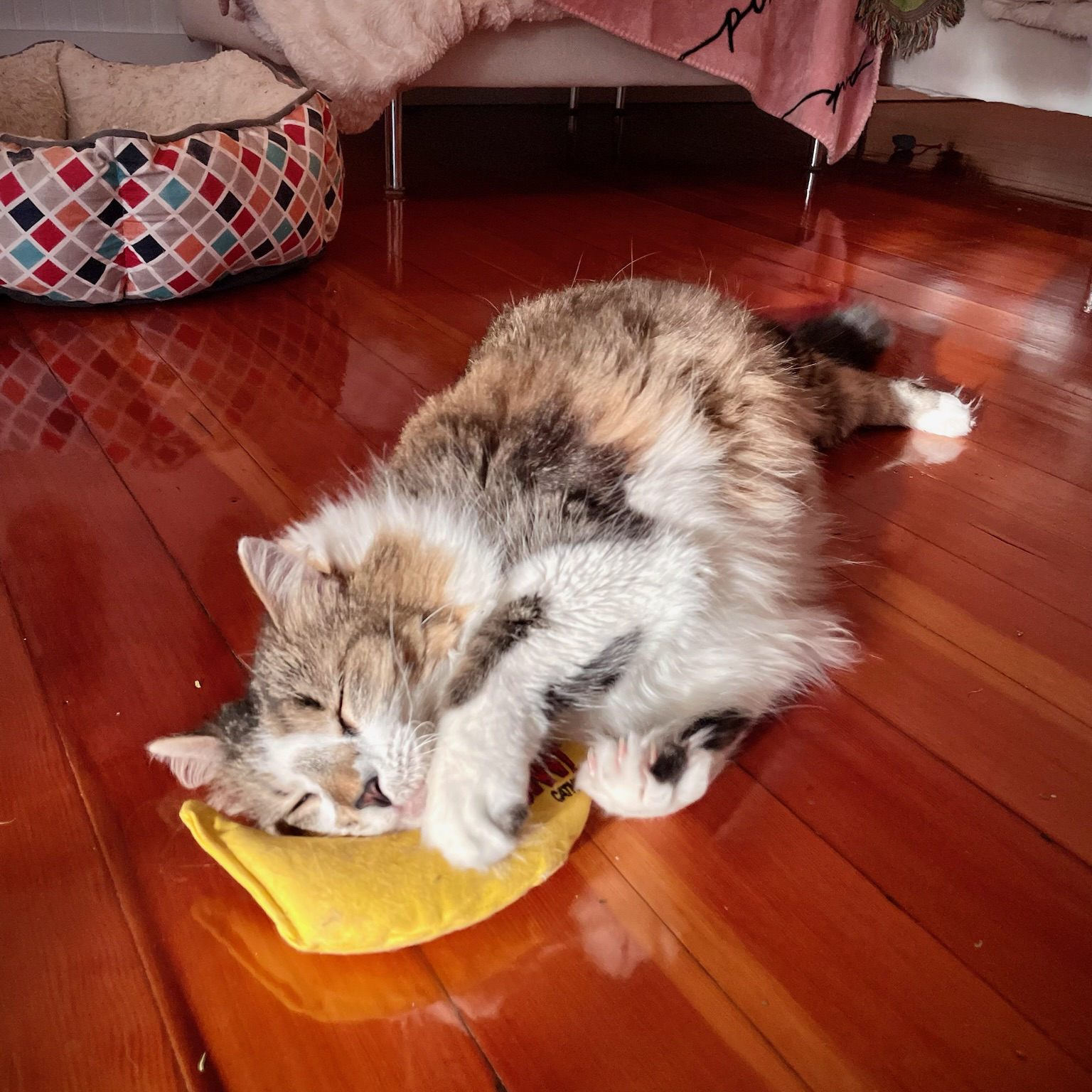
Likes
- Food
- Belly rubs
- Being alone with you
Dislikes
- Not getting food
- Being picked up
- Petting in ears
Favorite Spots
- Under the main bed
- In the main bedroom closet
- Under blankets on the couch/bed
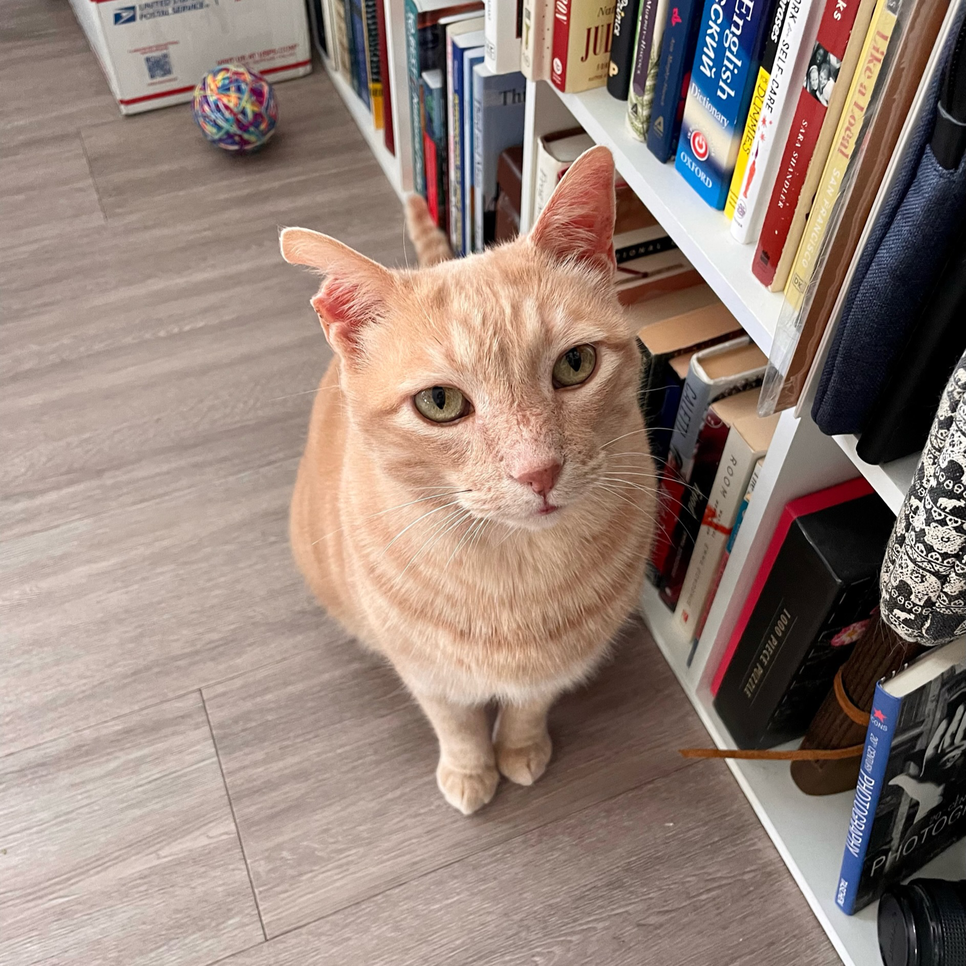
Birthday May 3rd, 2011
Nicknames Mr. Bodie, Bad Cat, Orange Cat
Bodie came into my life after my partner’s parents retired. They asked if we wanted him, and we said “Of course”.
At first, it was not an easy transition. He didn’t get along with Mallory. He gets upset in the middle of the night and cries. He gets upset in the middle of the day and cries.
But now he is an integral part of this family.
Likes
- Sous-vide meats, chicken, steak, etc.
- Being near people
- Being outside
- Back scratches and cuddles
- Play time with the chaser toys
- Thinking about quantum electrodynamics
Dislikes
- Not getting his way
- Being alone
Favorite Spots
- On blankets
- On the couch, on the arm rest
- In the living room cat tree/perch