
Illya Starikov

I hate this time of year.
There is a strange part of me deep down that knows it’s time. Time to mourn. Time to have anxiety. Time to feel not in control.
2022 was the worst year in many of our lives. Every year I do my best to pull myself together, bit my bit. And I largely succeed, until February.
Every February I start feeling in control, but come March I’m in a much worse place. It’s a force that drags me under and keeps me there.
Now that 2.24 has passed, I find myself picking up the pieces. Like last year. Like the year before.
Hello👋 I’m Illya Starikov. Welcome to my personal blog.
Over the years, I’ve made many iterations of blogs. Blogs about Apple, technology, programming, portfolios, entertainment. This one is just about me.
My interests, that I will likely write about, include:
- Cats
- Programming
- Technology
- Traveling
- Video games
- Running, lifting, basketball
- Photography
Hope you enjoy!
There is no greater agony than bearing an untold story inside you. Maya Angelou
Google Beam
Feel like you're there, together.
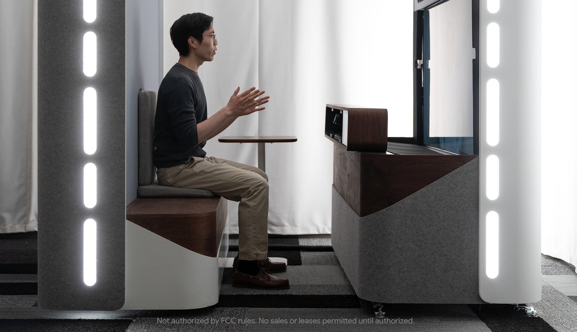
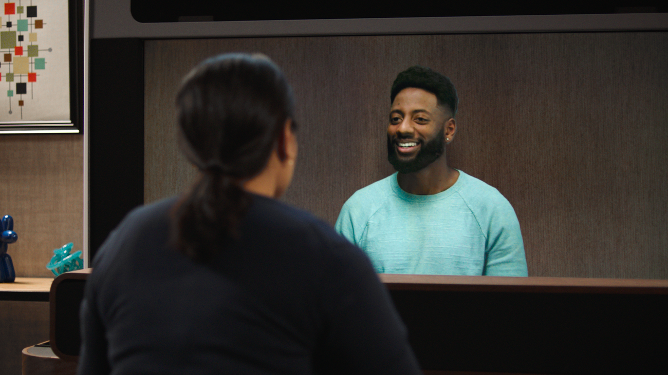
Google Project Starline is an experimental 3D telepresence system designed to make video calls feel as natural as face-to-face conversations. First unveiled in 2021, it combines advanced hardware and software to create a “magic window” effect – users on a Starline call see each other life-size and in three dimensions, as if they’re together in the same room. The goal is to bridge physical distance and help people (from coworkers to family members) feel truly present with each other, even when they are cities or countries apart.
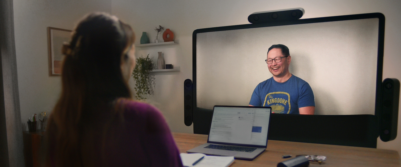
Project Starline uses a mix of 3D imaging, AI, spatial audio, and a special light-field display to produce its lifelike communication experience. Multiple cameras and sensors capture a person’s shape and movements from different angles, and Google’s systems process this data in real-time. The other user sees a life-size, three-dimensional image of the person on a large light-field screen, which creates an illusion of depth without the need for any VR headsets or glasses. This setup lets participants talk, gesture, and make eye contact naturally through the display, with spatial speakers recreating sound as if it’s coming from the person’s direction. In practice, it feels like sitting across from someone at a table – the technology fades into the background, and the conversation feels remarkably immersive and natural.
Project Starline is still in the prototype stage, but it has made notable progress. Initially the system was confined to a few Google offices, relying on custom-built equipment and even a booth-like enclosure. Googlers spent thousands of hours testing it internally, and early demos with select partners showed promise – participants found that meetings in Starline felt much more like real in-person meetings than traditional video calls, with better attentiveness and engagement. In late 2022, Google expanded testing through an early access program, installing Starline prototypes at partner organizations like Salesforce, T-Mobile, WeWork, and a healthcare network, to gather feedback in real workplace scenarios. A major breakthrough came in 2023 when Google unveiled a new, streamlined Starline prototype. Thanks to AI techniques that reduce the need for specialized cameras and depth sensors, the system shrank from the size of a restaurant booth to something resembling a large flat-screen TV. This slimmer design can more easily fit into offices or conference rooms, bringing Starline closer to a practical product.
Google is now preparing to bring Project Starline out of the lab and into broader use. In 2024, the company announced a partnership with HP to commercialize Starline, with plans to make it available to enterprise customers starting in 2025. The goal is to integrate Starline’s 3D calling experience with everyday video conferencing tools like Google Meet and Zoom, so that companies can use it for realistic remote meetings via familiar platforms. Early interest has come from a range of industries – Google has demoed Starline to partners in fields like healthcare, media, and retail, hinting at potential uses from telemedicine consultations to virtual retail experiences. Over time, as the technology becomes more affordable and accessible, it could also be used for personal communication (for example, helping families connect across long distances) and educational or training settings. Project Starline offers a glimpse into the future of remote communication, one where distance is less of a barrier and people can “be there” for important moments without having to travel.


GDL-60
Streamline your flight prep, and enjoy your aircraft more with the GDL 60 datalink and PlaneSync™ technology.

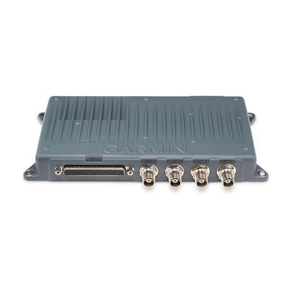
The Garmin GDL-60 is a small panel-mounted datalink module that brings wireless connectivity to an aircraft’s avionics suite. It is part of Garmin’s PlaneSync “connected cockpit” system and works with Garmin avionics (such as GTN™ Xi navigators and G1000®/G1000 NXi flight decks) to connect the aircraft to the outside world. In practice the GDL-60 acts like an onboard “internet box,” using both a built-in 4G LTE cellular modem and Wi‑Fi radio to link the plane’s systems with Garmin’s cloud services and pilot tablets. This lets the avionics exchange data automatically – for example, it can download chart and database updates or stream weather and traffic directly into mobile apps – without a pilot having to plug in data cards.
Technically, the GDL-60 is a compact device (about 8.72″ x 4.00″ x 1.12″ and 1.5 lb) that mounts in the instrument panel. It runs on 14/28 V DC aircraft power and is certified for high altitudes up to 55,000 ft. Its hardware includes dual Wi-Fi radios (one access point, one client) using 802.11 b/g/n at 2.4 GHz, plus a multi-band LTE modem covering global 4G frequencies. In effect, the GDL-60 creates both an onboard Wi‑Fi network and a cellular data link. The aircraft can thus stay connected on the ground or in flight, subject to cell coverage. Garmin’s documentation notes that the unit “enables PlaneSync technology” via these connections and that its LTE/Wi-Fi link automatically keeps the avionics databases updated.
Once installed, the GDL-60 offers several key features for pilots. One major advantage is automated database updates: Garmin explains that the GDL-60 “offers database downloads directly to the aircraft,” so that new charts and navigation data can download over the air without a pilot present. The system then “auto-synchronize[s] across your avionics at power up,” eliminating manual update chores. The GDL-60 also logs flight and engine data; after landing it can “transmit flight and engine log data automatically… to secure cloud storage,” where pilots or maintenance crews can review it via the Garmin Pilot mobile app or the flyGarmin web portal. Another useful feature is remote aircraft monitoring: with the GDL-60 and Garmin Pilot, an owner on the ground can check the airplane’s status from anywhere. The Pilot app can show things like Hobbs and tach times, fuel quantity, battery voltage, outside-air temperature, oil temperature, and even the last known GPS location of the aircraft. In short, GDL-60 keeps pilots informed about their aircraft’s health and readiness.
Perhaps the most visible benefit is mobile connectivity. The GDL-60 enables Garmin’s Connext system, which streams in-flight data from the panel to pilot devices. For example, it can send ADS-B weather (FIS-B) and traffic, GPS position, and even attitude (AHRS) information to apps like Garmin Pilot or ForeFlight. In fact, Garmin describes that the GDL-60 lets you “stream weather, traffic, AHRS, flight plans and other data from your avionics to flight apps such as Garmin Pilot and ForeFlight”. Pilots can also transfer flight plans between their tablet and the panel through this link. (With additional hardware, the GDL-60 can even extend to cabin entertainment and SATCOM: for example, pairing it with a SiriusXM receiver enables XM audio tuning via the Pilot app, and it can interface with a Garmin GSR-56 for in-flight texting/voice calls.) Overall, the Garmin GDL-60 turns a compatible cockpit into a connected cockpit – keeping nav databases current and putting real-time flight and weather data into pilots’ hands through familiar mobile interfaces.
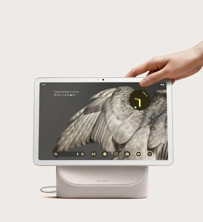
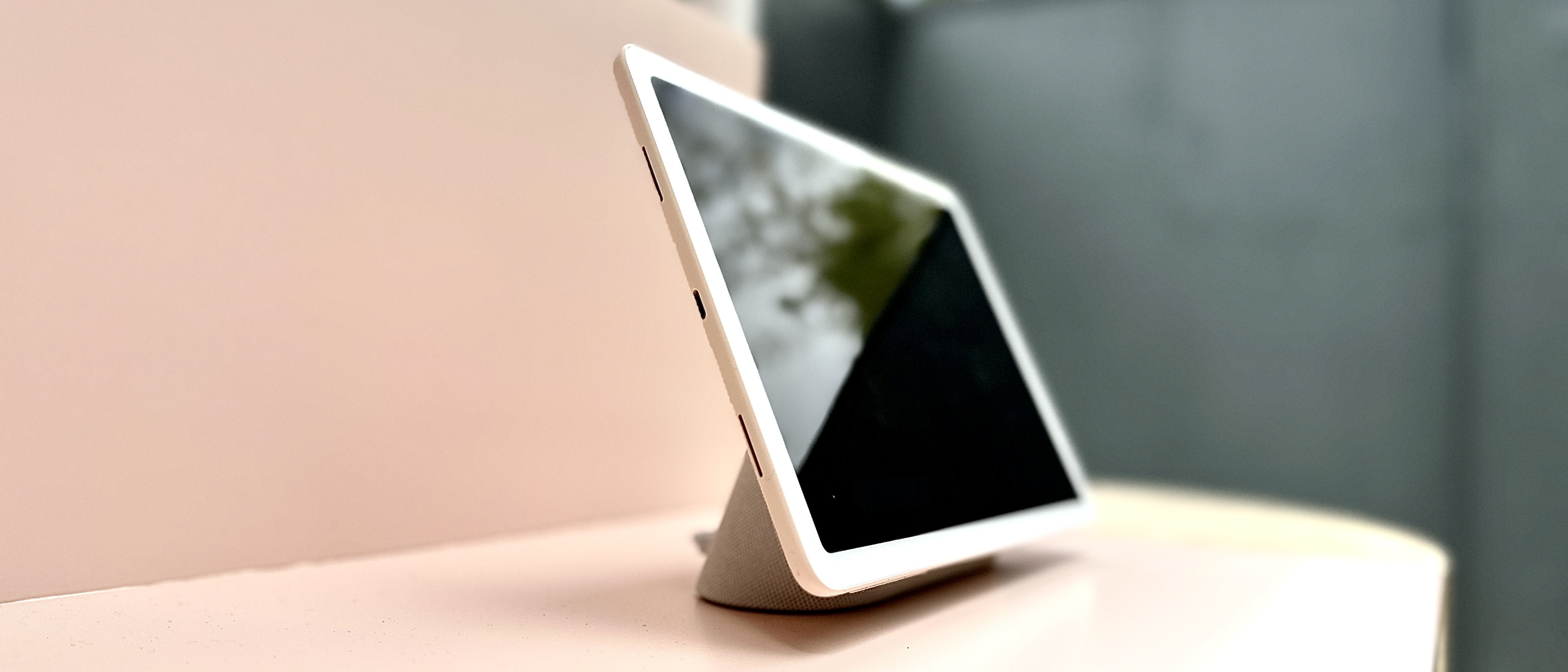
Pixel Tablet
Meet the new Google Pixel Tablet that’s helpful in your hands and at home.
The Google Pixel Tablet is a home-focused Android tablet released in 2023. It features a 10.95-inch LCD touchscreen display (2560 × 1600 resolution, 16:10 aspect ratio) with around 500 nits of brightness. The tablet’s build uses an aluminum frame with rounded edges and a nano-ceramic coating inspired by porcelain, which gives it a soft matte texture for better grip. Google offers the Pixel Tablet in three colors – Porcelain (off-white), Hazel (gray-green), and Rose (pink). The device also houses four built-in speakers (two on each side) for stereo audio output during media playback.
Under the hood, the Pixel Tablet is powered by Google’s Tensor G2 chipset (the same processor used in the Pixel 7 series smartphones). It comes with 8 GB of RAM and either 128 GB or 256 GB of internal UFS 3.1 storage (non-expandable). The tablet ships with Android 13 and includes Google’s Titan M2 security chip, with Google promising at least five years of security updates for the device. Power is supplied by a built-in 27 Wh battery (about 7020 mAh) that is rated for up to 12 hours of video streaming on a full charge. Connectivity is Wi‑Fi 6 and Bluetooth 5.2 only (the Pixel Tablet does not offer cellular/LTE support). For cameras, it has an 8 MP front camera and an 8 MP rear camera, both with fixed focus and primarily intended for video calls or simple photos. A fingerprint scanner is integrated into the power button for secure unlocking.
Google has optimized the Pixel Tablet’s software for a large screen experience. Many popular apps (such as YouTube, Spotify, and Disney+) have improved layouts on the tablet’s display, and a Google TV app comes preloaded to make it easy to browse and stream video content on the big screen. The tablet supports multitasking features like split-screen mode, allowing two apps to run side by side, and it offers accurate voice typing and other Google AI features for convenient hands-free input. It is also compatible with USI 2.0 stylus pens, enabling users to draw or take notes with a supported active stylus (no stylus is included in the box). Notably, the Pixel Tablet supports multiple user profiles – each family member can have their own account with separate apps, settings, and personalizations on the device. This multi-user support underlines its role as a shared home tablet.
One of the Pixel Tablet’s signature features is its Charging Speaker Dock, which comes included with the tablet. The tablet can be placed on this dock via pogo pin connectors (held in place magnetically), which both charges the device and boosts its audio. The dock contains a full-range speaker that provides significantly more bass and room-filling sound compared to the tablet’s built-in speakers. When the Pixel Tablet is docked, it automatically enters Hub Mode, functioning like a smart display for the home. In this mode, the tablet can show a hands-free Google Assistant interface, smart home controls, and even a digital photo frame or clock on the screen. Users can control smart devices (lights, thermostats, doorbells, etc.) directly from the tablet’s hub interface, similar to a Google Nest Hub. Additionally, the Pixel Tablet is the first tablet with Chromecast built-in, allowing you to cast music or videos from your phone to the tablet’s screen when it’s on the dock. This dual functionality lets the Pixel Tablet serve as both a personal tablet and a communal smart home display depending on how it’s being used.
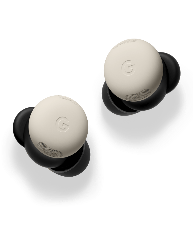
Pixel Buds Pro (I & II)
Loud and clear, Pixel Buds Pro are here.
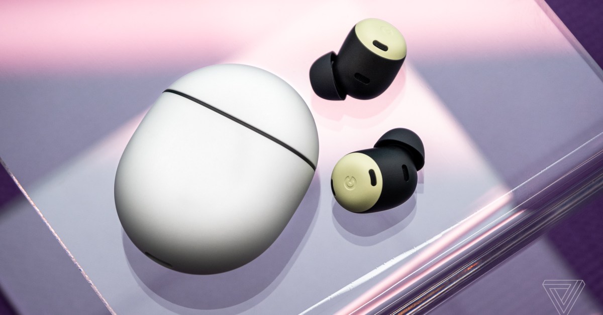
Google’s Pixel Buds Pro (released mid-2022) are compact true wireless earbuds with a smooth, stemless design. Unlike earlier Pixel Buds models, the Pro version drops the “stabilizer arc” wing-tips for a simpler in-ear fit, improving comfort. Each earbud comes with silicone tips in multiple sizes to ensure a snug seal. The oval charging case (available in four colors) has a pebble-like shape similar to the Pixel Buds A-Series case (about 10–15% larger). Both the earbuds and case are water-resistant (buds IPX4, case IPX2), making them suitable for workouts and light rain.
The Pixel Buds Pro include:
- Active Noise Cancellation (ANC) and a transparency (ambient sound) mode, letting you either block out or hear surrounding noise as needed.
- Hands-free Google Assistant for voice commands (play/pause, volume, etc.) and even on-device translation support in conversation mode.
- Multipoint Bluetooth pairing (connect to two devices at once) and Google Fast Pair for quick setup between phones, tablets, and laptops.
- Water/sweat resistance (earbuds rated IPX4) for use during exercise or in light rain.
The Pixel Buds Pro deliver strong audio and reliable performance. Reviewers note clear, well-balanced sound and effective noise canceling. They also feature an in-ear detection sensor that automatically pauses audio when you remove an earbud. Battery life is rated up to about 7 hours per charge with ANC on (11 hours with it off), and the compact case provides roughly two full extra charges (around 30 total hours). The case supports both USB-C wired charging and Qi wireless charging. Connectivity is much improved over earlier Pixel Buds: the earbuds use Bluetooth 5.0 with Google’s Fast Pair and show virtually no dropouts in testing. They also support automatic device switching (multipoint pairing) between two connected devices.


)
Nest Indoor Camera
Nest Cam tells you more about what’s going on inside.
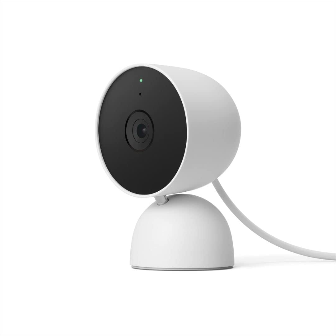
Google’s Nest Indoor Camera is a small home security camera designed for indoor use. It has a compact, rounded body and comes in neutral colors so it can blend into home decor. The camera can sit on a shelf or table using its built-in stand, or be mounted on a wall with the included bracket and screws. It connects to your home Wi-Fi network and streams live video to your smartphone or tablet through the Google Home app.
The camera records full high-definition (1080p) video and uses a wide-angle lens (about 135 degrees) to capture a broad area. It also uses high-dynamic-range (HDR) imaging to improve detail in bright and dark parts of the scene, and it has infrared night vision to see clearly even in low light. A built-in microphone and speaker allow two-way communication through the app, so you can listen to and speak with people or pets near the camera. Together, these video and audio features let you keep an eye on a room and even interact with anyone there while you’re away.
One of the camera’s key smart features is motion detection. If the camera detects movement, it automatically sends an alert to your phone. You can then open the live video feed in the Google Home app at any time to check on what’s happening. The camera also has a small LED light (usually green) that turns on when it is recording or streaming. This visual indicator lets people nearby know the camera is active and helps address privacy concerns.
Setup is straightforward and user-friendly. You plug the camera into a standard wall outlet using the supplied USB cable, then open the Google Home app on your phone to complete the setup. The app guides you through connecting the camera to your Wi-Fi network and naming the device, so most people can have it running in just a few minutes. This simple process means advanced technical skills are not needed to start using the camera.
As a product, the Nest Indoor Camera adds to Google’s Nest line of smart home security devices. It expands Google’s offerings for indoor monitoring and reinforces the company’s presence in the home security market. Overall reception has been positive, with many users praising its reliable performance, easy setup, and clean, modern design. Many also appreciate its smooth integration with Google’s smart home ecosystem, making it a convenient choice for monitoring a home.
The following is my goodbye email to Garmin, with names censored.
I joined Garmin in 2017, during my junior year of college. Bright eyed and bushy tailed, I drove to Los Angeles for my first internship at the Los Angeles office. It was an awesome opportunity, and I can’t thank S.S. enough for it.
Shortly after, I joined the Rolla office under T.S. I got my first taste of aviation software, working on an uncertified tool for Interfaces. I learned a lot from my mentor, A.H., and just as much from an unofficial mentor, B.B. A year had passed, and I started full time; but T.S. stayed a mentor to me since.
I started on M.T.'s team in June of last year. My only hardware experience was making lights blink on a microcontroller from the 80s and wiring a 10U nano-satellite to be launched off the ISS, so there was a bit of a knowledge gap. But my awesome team took me in, showed me the ropes, and only made fun of me a little. I learned several ways to do many things, and many ways to not do several things.
All in all, Garmin has been an incredible journey.
I want to thank my awesome team, both hardware and software, for always being dependable and knowledgable. I want to thank V.R. for keeping the project on track. I want to thank R.S., for being such an ace officemate/mentor/friend, and being so incredibly resilient to strobe lights and loud EDM music. I want to thank M.T. and T.S., for taking me in and giving me this incredible opportunity.
And I want to thank you, for making Garmin so memorable. :)