Computer Science

The ideas under the software: algorithms, theory, and the comforting news that the fundamentals never really change.

Sorting Algorithms

sort<Algorithm>(from: bubble, to: Tim)

INITIALIZING...

ALGORITHM

ARRAY SIZE

ARRAY PATTERN

THEME

CUSTOM ARRAY (OPTIONAL)

ANIMATION SPEED 50%

Enter Start

Space Pause

Esc Reset

High array size may impact performance

Select Algorithm

READY TO VISUALIZE

Time: 0.000s

Comparisons: 0

Swaps: 0

WAITING TO START

When I was a Teacher Assistant (TA) in Intro To Computer Science lab, fellow TA
Ian and I were showing off our programming prowess. I thought I had it in the bag: I had solved a competitive programming problem in compile-time (C++ templates are Turing-complete!) and a Space Invaders clone for a class.

But Ian was more clever than I, and showed me something that fundamentally changed how I saw a core-component of programming: a terminal-based (ncurses) sorting algorithm visualizers.
It was the first time I had ever seen these algorithms graphed like this — ever! And, yes, I blame my Algorithm instructor. I finally could see all the hypothetical sorting in a real-life application.

With the power of LLMs in hand, and a website as my canvas, I wanted to see if I could recreate this. Kudos to you, Ian.

Sorting algorithms form the backbone of computer science, serving as fundamental building blocks for countless applications from database management to search engines. This comprehensive guide examines the 25 most important sorting algorithms, organized by type, with detailed analysis of their performance, implementation, and practical applications.

1. Basic Comparison-Based Algorithms

These fundamental algorithms serve as the foundation for understanding sorting concepts, though they generally have O(n²) time complexity.

1.1 Bubble Sort

Complexity Analysis:

Best Case: O(n) / Ω(n) - when array is already sorted
Average Case: O(n²) / Θ(n²)
Worst Case: O(n²)
Space: O(1)

Properties: Stable, In-place, Adaptive

def bubble_sort(arr):
    """
    Bubble Sort with optimization
    Time: O(n²) average/worst, O(n) best
    Space: O(1)
    """
    n = len(arr)

    for i in range(n):
        swapped = False

        # Last i elements are already sorted
        for j in range(0, n - i - 1):
            if arr[j] > arr[j + 1]:
                arr[j], arr[j + 1] = arr[j + 1], arr[j]
                swapped = True

        # If no swapping occurred, array is sorted
        if not swapped:
            break

    return arr

When to Use:

Small datasets (< 50 elements)
Educational purposes - excellent for teaching
Nearly sorted data
Memory-constrained environments

Step-by-Step Example:
Array: [64, 34, 25, 12, 22, 11, 90]

Pass 1: [34, 25, 12, 22, 11, 64, 90] - Largest element "bubbles" to end
Pass 2: [25, 12, 22, 11, 34, 64, 90]
... continues until sorted

History: First described by Edward Harry Friend in 1956. The name "bubble sort" was coined by Kenneth E. Iverson due to how smaller elements "bubble" to the top.

Notable Trivia: Donald Knuth famously stated "bubble sort seems to have nothing to recommend it, except a catchy name." Despite criticism, it remains the most taught sorting algorithm due to its simplicity.

1.2 Selection Sort

Complexity Analysis:

Best/Average/Worst Case: O(n²) - always makes same comparisons
Space: O(1)

Properties: Unstable, In-place, Not adaptive

def selection_sort(arr):
    """
    Selection Sort implementation
    Time: O(n²) for all cases
    Space: O(1)
    """
    n = len(arr)

    for i in range(n):
        # Find minimum element in remaining unsorted array
        min_idx = i

        for j in range(i + 1, n):
            if arr[j] < arr[min_idx]:
                min_idx = j

        # Swap the found minimum element
        arr[i], arr[min_idx] = arr[min_idx], arr[i]

    return arr

When to Use:

When memory write operations are expensive (e.g., flash memory)
Small datasets where simplicity matters
When the number of swaps needs to be minimized

Key Advantage: Performs only O(n) swaps compared to O(n²) for bubble sort.

History: Has ancient origins in manual sorting processes. Formalized in the 1950s as one of the fundamental sorting methods.

1.3 Insertion Sort

Complexity Analysis:

Best Case: O(n) - already sorted
Average/Worst Case: O(n²)
Space: O(1)

Properties: Stable, In-place, Adaptive, Online

def insertion_sort(arr):
    """
    Insertion Sort implementation
    Time: O(n²) average/worst, O(n) best
    Space: O(1)
    """
    for i in range(1, len(arr)):
        key = arr[i]
        j = i - 1

        while j >= 0 and arr[j] > key:
            arr[j + 1] = arr[j]
            j -= 1

        arr[j + 1] = key

    return arr

When to Use:

Small datasets (typically < 50 elements)
Nearly sorted data - performs in O(n) time
Online algorithms - when data arrives sequentially
As a subroutine in quicksort and mergesort for small subarrays

Notable Use: Used in Timsort (Python's built-in sort) for small runs. Often faster than O(n log n) algorithms for arrays with fewer than 10-20 elements.

1.4 Shell Sort

Complexity Analysis:

Best Case: O(n log n)
Average Case: O(n^1.25) to O(n^1.5) depending on gap sequence
Worst Case: O(n²) for Shell's original sequence
Space: O(1)

Properties: Unstable, In-place, Adaptive

def shell_sort(arr):
    """
    Shell Sort using Shell's original sequence
    Time: O(n²) worst case, O(n log n) average
    Space: O(1)
    """
    n = len(arr)
    gap = n // 2

    while gap > 0:
        # Perform gapped insertion sort
        for i in range(gap, n):
            temp = arr[i]
            j = i

            while j >= gap and arr[j - gap] > temp:
                arr[j] = arr[j - gap]
                j -= gap

            arr[j] = temp

        gap //= 2

    return arr

When to Use:

Medium-sized datasets (100-5000 elements)
When recursion should be avoided
Embedded systems - simple and efficient

History: Invented by Donald L. Shell in 1959, it was one of the first algorithms to break the O(n²) barrier.

1.5 Cocktail Shaker Sort (Bidirectional Bubble Sort)

Complexity Analysis:

Best Case: O(n)
Average/Worst Case: O(n²)
Space: O(1)

Properties: Stable, In-place, Adaptive, Bidirectional

def cocktail_shaker_sort(arr):
    """
    Cocktail Shaker Sort (Bidirectional Bubble Sort)
    Time: O(n²) average/worst, O(n) best
    Space: O(1)
    """
    n = len(arr)
    start = 0
    end = n - 1

    while start < end:
        swapped = False

        # Forward pass
        for i in range(start, end):
            if arr[i] > arr[i + 1]:
                arr[i], arr[i + 1] = arr[i + 1], arr[i]
                swapped = True

        if not swapped:
            break

        end -= 1
        swapped = False

        # Backward pass
        for i in range(end, start, -1):
            if arr[i] < arr[i - 1]:
                arr[i], arr[i - 1] = arr[i - 1], arr[i]
                swapped = True

        if not swapped:
            break

        start += 1

    return arr

Advantage: Better than bubble sort at moving small elements (turtles) to the beginning.

2. Efficient Comparison-Based Algorithms

These algorithms achieve O(n log n) average performance and form the backbone of many practical sorting implementations.

2.1 Quick Sort

Complexity Analysis:

Best/Average Case: O(n log n)
Worst Case: O(n²) - when pivot is always minimum/maximum
Space: O(log n) - recursion stack

Properties: Unstable, In-place, Not adaptive

def quicksort(arr, low=0, high=None):
    """
    Quicksort with Hoare partition scheme
    Time: O(n log n) average, O(n²) worst
    Space: O(log n)
    """
    if high is None:
        high = len(arr) - 1

    if low < high:
        pivot_idx = partition(arr, low, high)
        quicksort(arr, low, pivot_idx)
        quicksort(arr, pivot_idx + 1, high)

    return arr

def partition(arr, low, high):
    """Hoare partition scheme"""
    pivot = arr[low]
    i = low - 1
    j = high + 1

    while True:
        i += 1
        while arr[i] < pivot:
            i += 1

        j -= 1
        while arr[j] > pivot:
            j -= 1

        if i >= j:
            return j

        arr[i], arr[j] = arr[j], arr[i]

Why It's Preferred Despite O(n²) Worst Case:

Excellent average-case performance with good constant factors
Cache-friendly sequential access patterns
In-place sorting
Modern implementations use introsort to guarantee O(n log n)

History: Invented by Tony Hoare in 1959 while working on machine translation at Moscow State University.

2.2 Merge Sort

Complexity Analysis:

All Cases: O(n log n) - guaranteed performance
Space: O(n) - requires additional space for merging

Properties: Stable, Not in-place, Not adaptive

def merge_sort(arr):
    """
    Merge Sort implementation
    Time: O(n log n) guaranteed
    Space: O(n)
    """
    if len(arr) <= 1:
        return arr

    mid = len(arr) // 2
    left = merge_sort(arr[:mid])
    right = merge_sort(arr[mid:])

    return merge(left, right)

def merge(left, right):
    """Merge two sorted arrays"""
    result = []
    i = j = 0

    while i < len(left) and j < len(right):
        if left[i] <= right[j]:
            result.append(left[i])
            i += 1
        else:
            result.append(right[j])
            j += 1

    result.extend(left[i:])
    result.extend(right[j:])

    return result

When to Use:

When stability is required
External sorting (large datasets that don't fit in memory)
Linked lists (efficient with O(1) extra space)
Parallel processing

History: Invented by John von Neumann in 1945, with detailed analysis published in 1948.

2.3 Heap Sort

Complexity Analysis:

All Cases: O(n log n) - guaranteed performance
Space: O(1) - true in-place sorting

Properties: Unstable, In-place, Not adaptive

def heap_sort(arr):
    """
    Heap Sort implementation
    Time: O(n log n) guaranteed
    Space: O(1)
    """
    n = len(arr)

    # Build max heap
    for i in range(n // 2 - 1, -1, -1):
        heapify(arr, n, i)

    # Extract elements from heap
    for i in range(n - 1, 0, -1):
        arr[0], arr[i] = arr[i], arr[0]
        heapify(arr, i, 0)

    return arr

def heapify(arr, n, i):
    """Maintain heap property"""
    largest = i
    left = 2 * i + 1
    right = 2 * i + 2

    if left < n and arr[left] > arr[largest]:
        largest = left

    if right < n and arr[right] > arr[largest]:
        largest = right

    if largest != i:
        arr[i], arr[largest] = arr[largest], arr[i]
        heapify(arr, n, largest)

When to Use:

Memory-constrained environments
Real-time systems (guaranteed performance)
Systems concerned with malicious input

History: Invented by J. W. J. Williams in 1964, with in-place version by Robert Floyd.

2.4 Binary Tree Sort

Complexity Analysis:

Best/Average Case: O(n log n) - with balanced tree
Worst Case: O(n²) - with unbalanced tree
Space: O(n) - for tree structure

Properties: Can be stable, Not in-place

When to Use:

Educational purposes
When tree structure is needed for other operations
Online sorting

Note: Self-balancing trees (AVL, Red-Black) guarantee O(n log n) performance.

2.5 Smooth Sort

Complexity Analysis:

Best Case: O(n) - for sorted data
Average/Worst Case: O(n log n)
Space: O(1)

Properties: Unstable, In-place, Adaptive

History: Invented by Edsger W. Dijkstra in 1981 as an improvement over heapsort for partially sorted data.

Notable Use: Used in musl C library's qsort() implementation.

3. Non-Comparison Based Algorithms

These algorithms achieve linear O(n) time complexity by exploiting specific properties of the data rather than comparing elements.

3.1 Counting Sort

Complexity Analysis:

All Cases: O(n + k) where k is the range of values
Space: O(n + k)

Properties: Stable, Not in-place

def counting_sort(arr):
    """
    Counting Sort for non-negative integers
    Time: O(n + k)
    Space: O(n + k)
    """
    if not arr:
        return arr

    max_val = max(arr)
    count = [0] * (max_val + 1)

    # Count occurrences
    for num in arr:
        count[num] += 1

    # Calculate cumulative count
    for i in range(1, len(count)):
        count[i] += count[i - 1]

    # Build output array
    output = [0] * len(arr)
    for i in range(len(arr) - 1, -1, -1):
        output[count[arr[i]] - 1] = arr[i]
        count[arr[i]] -= 1

    return output

When to Use:

Sorting integers in a small range
As a subroutine in radix sort
When k is O(n) or smaller

History: Invented by Harold H. Seward in 1954 at MIT.

3.2 Radix Sort

Complexity Analysis:

All Cases: O(d × (n + k)) where d is number of digits
Space: O(n + k)

Properties:

LSD (Least Significant Digit): Stable
MSD (Most Significant Digit): Can be stable

def radix_sort_lsd(arr):
    """
    LSD Radix Sort implementation
    Time: O(d × (n + k))
    Space: O(n + k)
    """
    if not arr:
        return arr

    max_val = max(arr)
    exp = 1

    while max_val // exp > 0:
        counting_sort_for_radix(arr, exp)
        exp *= 10

    return arr

def counting_sort_for_radix(arr, exp):
    n = len(arr)
    output = [0] * n
    count = [0] * 10

    for i in range(n):
        index = arr[i] // exp
        count[index % 10] += 1

    for i in range(1, 10):
        count[i] += count[i - 1]

    i = n - 1
    while i >= 0:
        index = arr[i] // exp
        output[count[index % 10] - 1] = arr[i]
        count[index % 10] -= 1
        i -= 1

    for i in range(n):
        arr[i] = output[i]

When to Use:

Sorting integers with many digits
String sorting (MSD variant)
When d is small compared to log n

History: Dates back to 1887 with Herman Hollerith's tabulating machines.

3.3 Bucket Sort

Complexity Analysis:

Best/Average Case: O(n + k) for uniform distribution
Worst Case: O(n²) when all elements fall into one bucket
Space: O(n + k)

Properties: Stable (if sub-sorting is stable), Not in-place

def bucket_sort(arr):
    """
    Bucket Sort for floating-point number
    Time: O(n + k) average
    Space: O(n + k)
    """
    if not arr:
        return arr

    min_val, max_val = min(arr), max(arr)
    bucket_count = len(arr)
    buckets = [[] for _ in range(bucket_count)]

    # Distribute elements into buckets
    for num in arr:
        if max_val == min_val:
            index = 0
        else:
            index = int((num - min_val) / (max_val - min_val) * (bucket_count - 1))
        buckets[index].append(num)

    # Sort individual buckets
    result = []
    for bucket in buckets:
        if bucket:
            bucket.sort()  # Can use insertion sort
            result.extend(bucket)

    return result

When to Use:

Uniformly distributed floating-point numbers
Large datasets with known range
When memory is not a constraint

3.4 Pigeonhole Sort

Complexity Analysis:

All Cases: O(n + range) where range = max - min + 1
Space: O(range)

Properties: Stable, Not in-place

When to Use:

Small range of integer values
When range is comparable to n
Simple counting applications

History: Based on the pigeonhole principle, formally described by A.J. Lotka (1926).

3.5 Flash Sort

Complexity Analysis:

Best/Average Case: O(n) for uniform distribution
Worst Case: O(n²)
Space: O(m) where m is number of classes

Properties: Unstable, In-place (major advantage)

When to Use:

Large uniformly distributed datasets
When memory is limited
When O(n) average performance is critical

History: Invented by Karl-Dietrich Neubert in 1998 as an efficient in-place implementation of bucket sort.

4. Modern Hybrid Algorithms

These algorithms represent the state-of-the-art in practical sorting, combining multiple techniques for superior performance.

4.1 Timsort

Complexity Analysis:

Best Case: O(n) - already sorted
Average/Worst Case: O(n log n)
Space: O(n)

Properties: Stable, Not in-place

Key Innovations:

Run Detection: Identifies naturally occurring sorted subsequences
Minimum Run Size: Calculates optimal minrun (32-64 elements)
Galloping Mode: Switches to exponential search when one run consistently "wins"

Where It's Used:

Python's default sort since version 2.3
Java for sorting objects (Java 7+)
Android, V8, Swift, Rust

History: Created in 2002 by Tim Peters for Python. A critical bug was discovered and fixed in 2015 through formal verification.

4.2 Introsort (Introspective Sort)

Complexity Analysis:

All Cases: O(n log n) - guaranteed by heapsort fallback
Space: O(log n)

Properties: Unstable, In-place

Techniques Combined:

Quicksort for main sorting
Heapsort when recursion depth exceeds 2×log₂(n)
Insertion sort for small subarrays (< 16 elements)

Where It's Used:

C++ STL's std::sort() in GCC and LLVM
Microsoft .NET Framework 4.5+

History: Created by David Musser in 1997 to provide guaranteed O(n log n) performance while maintaining quicksort's average-case speed.

4.3 Block Sort (WikiSort)

Complexity Analysis:

Best Case: O(n)
Average/Worst Case: O(n log n)
Space: O(1) - constant space!

Properties: Stable, In-place

Key Innovation: Achieves stable merge sort performance with O(1) space by using internal buffering.

When to Use: When O(1) space complexity and stability are both required.

4.4 Pattern-defeating Quicksort (pdqsort)

Complexity Analysis:

Best Case: O(n) for specific patterns
Average/Worst Case: O(n log n)
Space: O(log n)

Properties: Unstable, In-place

Key Innovations:

Pattern detection and optimization
Branchless partitioning
Adaptive strategy based on input characteristics

Where It's Used:

Rust's default unstable sort
C++ Boost libraries

History: Created by Orson Peters in 2016 to improve upon introsort with better pattern handling.

4.5 Dual-Pivot Quicksort

Complexity Analysis:

Best Case: O(n) when all elements equal
Average Case: O(n log n) - 5% fewer comparisons than single-pivot
Worst Case: O(n²) - still possible but less likely
Space: O(log n)

Properties: Unstable, In-place

Key Innovation: Uses two pivots to partition array into three parts, reducing comparisons.

Where It's Used: Java's default algorithm for primitive arrays since Java 7.

History: Created by Vladimir Yaroslavskiy in 2009, adopted by Java in 2011.

5. Specialized and Educational Algorithms

These algorithms serve specific purposes or demonstrate important concepts in computer science education.

5.1 Comb Sort

Complexity Analysis:

Best Case: O(n log n)
Average Case: O(n²/2^p) where p is number of increments
Worst Case: O(n²)
Space: O(1)

Properties: Unstable, In-place

Key Feature: Improves upon bubble sort using variable gap with shrink factor of 1.3.

History: Developed by Włodzimierz Dobosiewicz in 1980 to address bubble sort's inefficiency.

5.2 Gnome Sort (Stupid Sort)

Complexity Analysis:

Best Case: O(n)
Average/Worst Case: O(n²)
Space: O(1)

Properties: Stable, In-place, Adaptive

Unique Feature: Uses only a single while loop - inspired by garden gnomes sorting flower pots.

5.3 Cycle Sort

Complexity Analysis:

All Cases: O(n²)
Space: O(1)

Properties: Unstable, In-place

Key Feature: Minimizes memory writes - each element is written at most once to its correct position.

When to Use: When memory write operations are expensive (EEPROM, Flash memory).

5.4 Pancake Sort

Complexity Analysis:

Best Case: O(n)
Average/Worst Case: O(n²)
Space: O(1)

Properties: Unstable, In-place

Unique Constraint: Only allowed operation is "flip" (reverse prefix).

Historical Note: Bill Gates' only published academic paper was on this problem (1979), providing a (5n+5)/3 upper bound algorithm.

5.5 Bogo Sort

Complexity Analysis:

Best Case: O(n) - already sorted
Average Case: O(n·n!) - expected permutations
Worst Case: O(∞) - theoretically unbounded
Space: O(1)

Properties: Unstable, In-place

Educational Value:

Demonstrates worst-case analysis
Teaches randomized algorithms
Shows importance of algorithm selection

import random

def bogo_sort(arr):
    """The worst sorting algorithm ever conceived"""
    def is_sorted(arr):
        return all(arr[i] <= arr[i+1] for i in range(len(arr)-1))

    while not is_sorted(arr):
        random.shuffle(arr)

    return arr

Trivia: "Quantum Bogo Sort" hypothetically destroys universes where array isn't sorted, leaving only sorted universes.

Summary and Recommendations

Performance Comparison Table

Algorithm	Best Case	Average Case	Worst Case	Space	Stable	In-Place
Bubble Sort	O(n)	O(n²)	O(n²)	O(1)	Yes	Yes
Selection Sort	O(n²)	O(n²)	O(n²)	O(1)	No	Yes
Insertion Sort	O(n)	O(n²)	O(n²)	O(1)	Yes	Yes
Quick Sort	O(n log n)	O(n log n)	O(n²)	O(log n)	No	Yes
Merge Sort	O(n log n)	O(n log n)	O(n log n)	O(n)	Yes	No
Heap Sort	O(n log n)	O(n log n)	O(n log n)	O(1)	No	Yes
Counting Sort	O(n+k)	O(n+k)	O(n+k)	O(n+k)	Yes	No
Radix Sort	O(d(n+k))	O(d(n+k))	O(d(n+k))	O(n+k)	Yes	No
Timsort	O(n)	O(n log n)	O(n log n)	O(n)	Yes	No

When to Use Which Algorithm

For Small Datasets (< 50 elements):

Insertion Sort - simple and efficient
Selection Sort - when minimizing swaps matters

For General Purpose:

Timsort (Python) or Introsort (C++) - best overall performance
Quick Sort with good pivot selection - excellent average case

For Guaranteed Performance:

Merge Sort - stable and predictable
Heap Sort - when O(1) space is required

For Special Data Types:

Counting Sort - small integer ranges
Radix Sort - large integers or strings
Bucket Sort - uniformly distributed floats

For Educational Purposes:

Start with Bubble Sort for simplicity
Progress to Quick Sort and Merge Sort
Use Bogo Sort to demonstrate algorithm analysis

Key Takeaways

No single best algorithm - choice depends on data characteristics, constraints, and requirements
Modern algorithms are hybrids - combining techniques yields superior performance
Stability matters for sorting complex objects where maintaining relative order is important
Space-time tradeoffs are crucial - some algorithms trade memory for speed
Real-world performance often differs from theoretical complexity due to cache effects, data patterns, and implementation details

Understanding these 25 algorithms provides a comprehensive foundation for tackling sorting problems in any context, from embedded systems to large-scale data processing.

Saturday, 22 November 2025

, & Illya Starikov

Computer Science Code Application AI Generated

The Zero-Width Space-Place

Nothing to see here.

Zero‑Width Space

Click the translucent pill (blue dot marks it) or the big Copy button.

What’s Zero-Width Space?

The zero‑width space (U+200B) is a Unicode glyph that renders nothing and occupies zero width. In the right hands, this “invisible ink” changes how software treats text.

Example

Below are seven tricks I actually use, each with a quick demo.

Anchor an Alphabetical List
Prefix one or more ZWS characters to push an item ahead of "A".

Newsletter  ← with ZWS
Apple
Zucchini

Break Auto‑Linking
Drop a ZWS into a URL or email to foil scrapers while leaving it human‑readable.

hello@starikov.co
https://starikov.co

Duplicate C++ Identifiers
ZWS is a valid identifier char in many compilers.

int total = 1;     // normal
int total = 2;     // looks the same, compiles fine
std::cout << total + total; // prints 3

Python Indentation Gremlins
Slip a ZWS into leading spaces; code looks aligned but crashes.

def hello():
    print("ok")   # four spaces
    print("boom") # four + ZWS → IndentationError

Hide Easter‑Egg Text
Insert a binary watermark every 100 chars; humans never see it, diff tools do.
Zero‑Length Social Forms
Some platforms allow a username, bios, and other forms that is literally just ZWS. Pure minimalism.
Control word‑wrapping
Add ZWS inside a super‑long URL to let browsers break the line without inserting a visible hyphen.

<span style="word-break:break-all">
    https://example.com/superlongpaththatneverends
</span>

Sunday, 18 May 2025

, & Illya Starikov

Technology Application Computer Science

Evolutionary Algorithms Endgame Dynamics

Adaptive Restarts and Termination Conditions

Update: Previously, a system was introduced for detecting if an individual was stuck at a local optimum. After extensive testing, this system was shown to be fragile. This post has been updated to showcase a more robust system.

Previously our Evolutionary Algorithms had it pretty easy: there would be either one local optimum (like our Secret Message problem instance) or multiple valid local optima (like the 3-SAT problem instance). In the real world, we might not be so lucky.

Often, an Evolutionary Algorithm might encounter a local optimum within the search space, and it will not be so easy to escape — offspring generated will be in close proximity of the optimum, and the mutation will not be enough to start exploring other parts of the search space.

To add to the frustration, there might not enough time or patience to wait for the Evolutionary Algorithm to finish. We might have different criteria we are looking for, outside of just a fitness target.

We are going to tackle both of these issues.

Applying Termination Conditions

First, we will examine what criteria we want met before our Evolutionary Algorithm terminates. In general, there are six that are universal:

Date and Time. After a specified date and time, terminate.
Fitness Target. This is what we had before; terminate when any individual attains a certain fitness.
Number of Fitness Evaluations. Every generation, every individual's fitness is evaluated (in our case, every generation $\mu + \lambda$ fitnesses are evaluated). Terminate after a specified number of fitness evaluations.
Number of Generations. Just like the number of fitness evaluations, terminate after a specified generations.
No Change In Average Fitness. This is a bit tricky. After specify $N$ generations, we check every $N$ generations back to determine if the average fitness of a population has improved. We have to be careful in our programming; by preserving diversity, we almost always lose fitness.
No Change In Best Fitness. Just like No Change In Average Fitness, but instead of taking the average fitness, we take the best.

Later, we will see how Conditions 5 & 6 will come in handy to determining if we are stuck in a local optimum.

To make sure we are always given valid termination conditions, we will have a super class that all termination conditions will inherit from. From there, we will have a separate condition for each of the listed conditions above.

class _TerminationCondition:
    pass

class FitnessTarget(_TerminationCondition):
    """Terminate after an individual reaches a particular fitness."""

class DateTarget(_TerminationCondition):
    """Terminate after a particular date and time."""

class NoChangeInAverageFitness(_TerminationCondition):
    """Terminate after there has been no change in the average
    fitness for a period of time."""

class NoChangeInBestFitness(_TerminationCondition):
    """Terminate after there has been no change in the best fitness
    for a period of time."""

class NumberOfFitnessEvaluations(_TerminationCondition):
    """Terminate after a particular number of fitness evaluations."""

class NumberOfGenerations(_TerminationCondition):
    """Terminate after a particular number of generations."""

Now, we need something that will keep track of all these conditions, and tells us when we should terminate. And here's where we need to be careful.

First, we need to know when to terminate. We want to mix and match different conditions, depending on the use case. This begs the questions:

Should the Evolutionary Algorithm terminate when one condition has been met, or all of them?

Generally, it makes more sense to terminate when any of the conditions have been met, as opposed to all of them. Suppose the two termination conditions are date and target fitness. It does not make sense to keep going after the target fitness is reached, and (if in a time crunch) it does not make sense to keep going after a specified date.

Second, how should we define no change in average/best fitness? These values can be quite sinusoidal, so we want to be more conservative in our definition. One plausible solution is to take the average of the first quartile (the first 25% to ever enter the queue), and see if the there is a single individual with a better fitness in the second, third, or fourth quartile (the last 75% percent to enter the queue). This way, even if there were very dominant individuals in the beginning, a single, more dominant individual will continue the Evolutionary Algorithm.

From this, we have everything we might need to keep track of our terminating conditions.

class TerminationManager:
    def __init__(self, termination_conditions, fitness_selector):
        assert isinstance(termination_conditions, list)
        assert all(issubclass(type(condition), _TerminationCondition)
                   for condition in termination_conditions), \
               "Termination condition is not valid"

        self.termination_conditions = termination_conditions
        self.__fitness_selector = fitness_selector

        self.__best_fitnesses = []
        self.__average_fitnesses = []

        self.__number_of_fitness_evaluations = 0
        self.__number_of_generations = 0

    def should_terminate(self):
        for condition in self.termination_conditions:
            if (isinstance(condition, FitnessTarget) and
                    self.__fitness_should_terminate()):
                return True
            elif (isinstance(condition, DateTarget) and
                    self.__date_should_terminate()):
                return True
            elif (isinstance(condition, NoChangeInAverageFitness) and
                    self.__average_fitness_should_terminate()):
                return True
            elif (isinstance(condition, NoChangeInBestFitness) and
                    self.__best_fitness_should_terminate()):
                return True
            elif (isinstance(condition, NumberOfFitnessEvaluations) and
                    self.__fitness_evaluations_should_terminate()):
                return True
            elif (isinstance(condition, NumberOfGenerations) and
                    self.__generations_should_terminate()):
                return True

        return False

    def reset(self):
        """Reset the best fitnesses, average fitnesses, number of
        generations, and number of fitness evaluations."""
        self.__best_fitnesses = []
        self.__average_fitnesses = []

        self.__number_of_fitness_evaluations = 0
        self.__number_of_generations = 0

    def __fitness_should_terminate(self):
        """Determine if should terminate based on the max fitness."""

    def __date_should_terminate(self):
        """Determine if should terminate based on the date."""

    def __average_fitness_should_terminate(self):
        """Determine if should terminate based on the average fitness
        for the last N generations."""

    def __best_fitness_should_terminate(self):
        """Determine if should terminate based on the average fitness
        for the last N generations."""

    def __fitness_evaluations_should_terminate(self):
        """Determine if should terminate based on the number of
        fitness evaluations."""

    def __generations_should_terminate(self):
        """Determine if should terminate based on the number of generations."""

And the changes to our Evolutionary Algorithm are minimal, too.

class EA:
    ...
    
    def search(self, termination_conditions):
        generation = 1
        self.population = Population(self.μ, self.λ)

        fitness_getter = lambda: [individual.fitness
                                  for individual
                                  in self.population.individuals]
        termination_manager = TerminationManager(termination_conditions,
                                                  fitness_getter)

        while not termination_manager.should_terminate():
            offspring = Population.generate_offspring(self.population)
            self.population.individuals += offspring.individuals
            self.population = Population.survival_selection(
                self.population)

            print("Generation #{}: {}".format(
                generation, self.population.fittest.fitness))
            generation += 1

        print("Result: {}".format(self.population.fittest.genotype))
        return self.population.fittest

However, we can still do better.

Generations Into Epochs

Before, the Evolutionary Algorithm framework we put in place was strictly a generational model. One generation lead to the next, and there were no discontinuities. Now, let's make our generational model into an epochal one.

We define an epoch as anytime our Evolutionary Algorithm encounters a local optimum. Once the end of an epoch is reached, the EA is reset, and the previous epoch is saved. Upon approaching the end of the next epoch, reintroduce the last epoch into the population; by this, more of the search space is covered.

How can we determine if we are at a local optimum?

We can't.

That does not mean we cannot have a heuristic for it. When there is little to no change in average/best fitness for a prolonged period of time, that typically means a local optimum has been reached. How long is a prolonged period of time? That's undetermined; it is another parameter we have to account for.

Note, if the Evolutionary Algorithm keeps producing more fit individuals, but the average fitness remains the same, the algorithm will terminate. Likewise, if the best fitness remains the same, but the average fitness closely approaches the best, the EA will terminate. Therefore, we should determine if the best fitness and the average fitness has not changed; only then should we start a new epoch.

Luckily, we already have something that will manage the average/best fitness for us.

class EA:
    ...

    def search(self, termination_conditions):
        epochs, generation, total_generations = 1, 1, 1
        self.population = Population(self.μ, self.λ)

        previous_epoch = []
        fitness_getter = lambda: [individual.fitness
                                  for individual
                                  in self.population.individuals]

        termination_manager = TerminationManager(termination_conditions,
                                                  fitness_getter)
        epoch_manager_best_fitness = TerminationManager(
            [NoChangeInBestFitness(250)], fitness_getter)
        epoch_manager_average_fitness = TerminationManager(
            [NoChangeInAverageFitness(250)], fitness_getter)

        while not termination_manager.should_terminate():
            if (epoch_manager_best_fitness.should_terminate() and
                    epoch_manager_average_fitness.should_terminate()):
                if len(previous_epoch) > 0:
                    epoch_manager_best_fitness.reset()
                    epoch_manager_average_fitness.reset()

                    self.population.individuals += previous_epoch
                    previous_epoch = []
                else:
                    epoch_manager_best_fitness.reset()
                    epoch_manager_average_fitness.reset()

                    previous_epoch = self.population.individuals
                    self.population = Population(self.μ, self.λ)

                    generation = 0
                    epochs += 1

            self.population = Population.survival_selection(self.population)

            offspring = Population.generate_offspring(self.population)
            self.population.individuals += offspring.individuals

            self.__log(total_generations, epochs, generation)

            total_generations += 1
            generation += 1

        print("Result: {}".format(self.population.fittest.genotype))
        return self.population.fittest


    def __log(self, total_generations, epochs, generation):
        """Log the process of the Evolutionary Algorithm."""
        ...

Although considerably more complicated, this new Evolutionary Algorithm framework allows us to explore much more of a search space (without getting stuck).

Let's put it to the test.

A New 3-SAT Problem

We're going to take on a substantially harder 3-SAT instance: 1,000 clauses, 250 variables. To make it worse, the number of valid solutions is also lower. We will also include the following terminating conditions:

Time of eight hours.
Fitness of all clauses satisfied (100).
A million generations.

So, how does our Evolutionary Algorithm fare?

Not well. After twenty epochs, and thousands of generations — we do not find a solution. Fear not; in subsequent posts, we will work on optimizing our Genetic Algorithm to handle much larger cases, more effectively.

Tuesday, 13 November 2018

, & Illya Starikov

AI Code Computer Science

Evolutionary Algorithms Recombination Operators

Permutation, Integer, and Real-Valued Crossover

We have been introduced to recombination operators before; however, that was merely an introduction. There are dozens of different Evolutionary Algorithm recombination operators for any established genotype; some are simple, some are complicated.

For a genotype representation that is a permutation (such as a vector^[1], bit-string, or hash-map^[2]), we have seen a possible recombination operator. Our 3-SAT solver uses a very popular recombination technique: uniform crossover.

Furthermore, we know a permutation is not the only, valid genotype for an individual: other possibilities can include an integer or a real-valued number.

Note, for simplicity, we will discuss recombination to form one offspring. This exact process can be applied to form a second child (generally with the parent's role reversed). Recombination can also be applied to more than two parents (depending on the operator). Again, for simplicity, we choose to omit it^[3].

First, let us start with permutations.

Permutation Crossover

In regard to permutation crossover, there are three common operators:

Uniform Crossover
$N$ -Point Crossover
Davis Crossover

Uniform crossover we have seen before. We consider individual elements in the permutation, and choose one with a random, equal probability. For large enough genotypes, the offspring genotype should consist of 50% of the genotype from parent one, and 50% of the genotype from parent two.

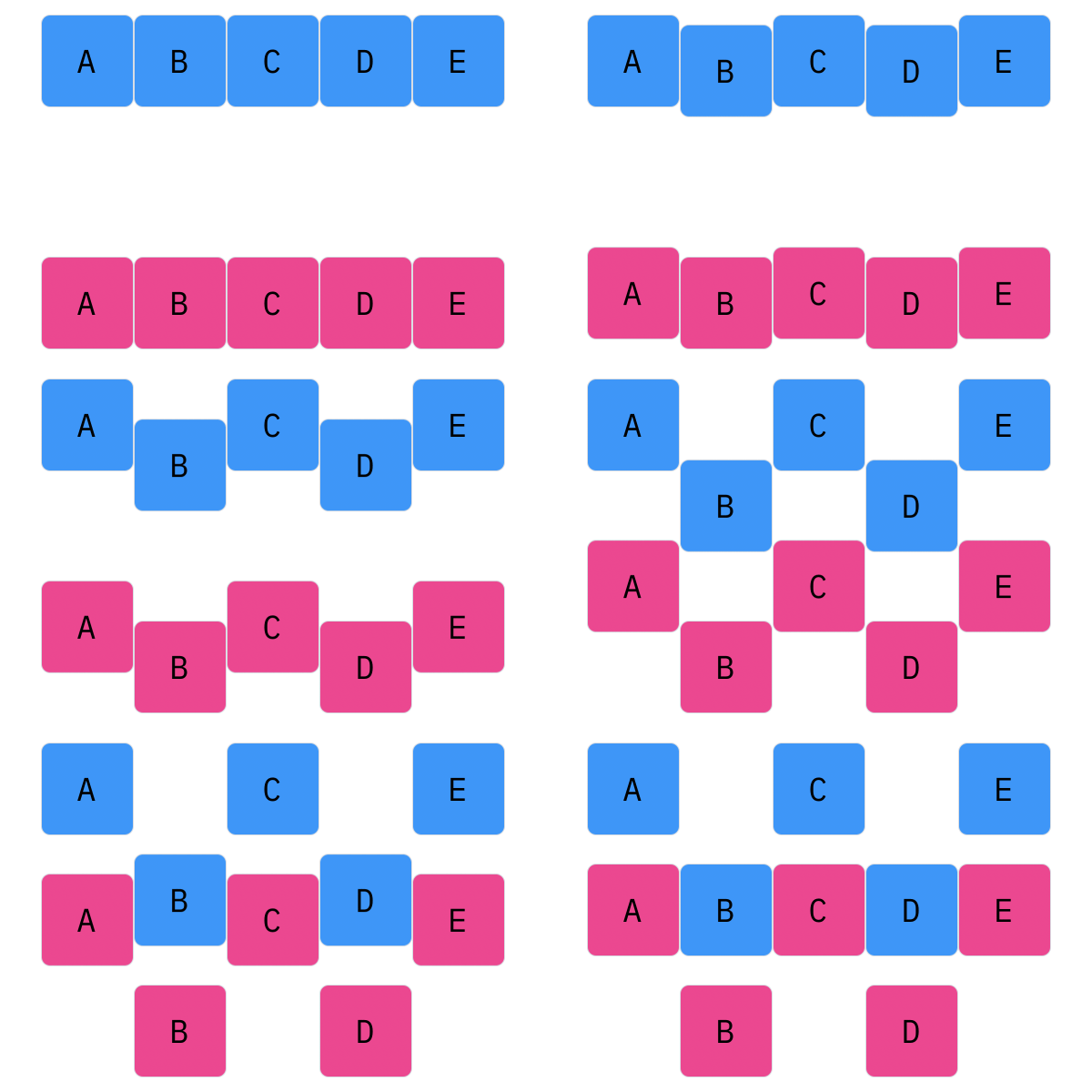
$N$-Point crossover considers segments of a genotype, as opposed to individual elements. This operator splits the genotype of Parent 1 and Parent 2 $N$ times (hence the name $N$-point), and creates a genotype by alternating segments from the two parents. For every $N$, there will be $N + 1$ segments. For 1-point crossover, the genotype should be split into two segments, and the offspring genotype should be composed of one segment from Parent 1, and one segment from Parent 2. For 2-point crossover, there will be three segments, and the offspring genotype will have two parts from Parent 1 and one part from Parent 2 (or two parts, Parent 1, one part, Parent 2).

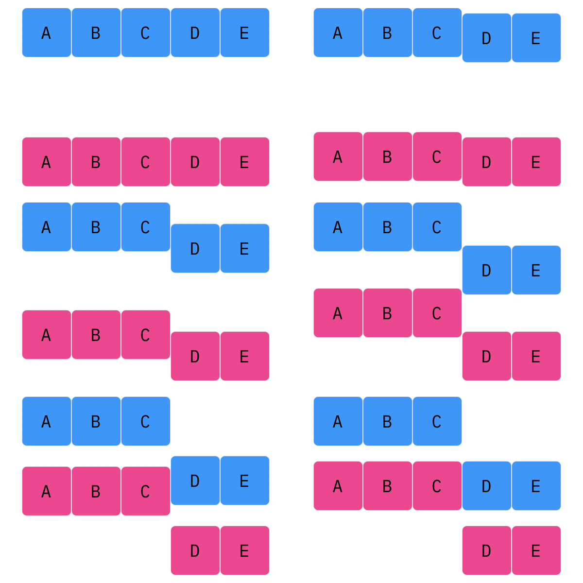
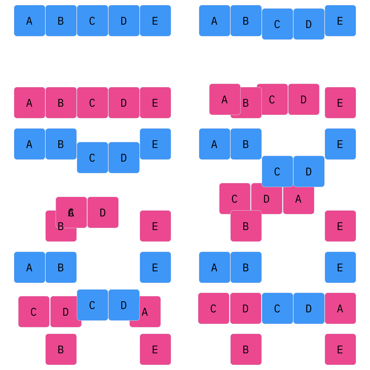
Davis Crossover tries to preserve the ordering of the genotype in the offspring (as opposed to the previous methods, where ordering was not considered). The premise is a bit complicated, but bear with me. Pick two random indices ($k_1$ and $k_2$), and copy the genetic material of Parent 1 from $k_1$ to $k_2$ into the offspring at $k_1$ to $k_2$. Put Parent 1 to the side, his role is finished. Start copying the genotype of Parent 2 starting at $k_1$ to $k_2$ at the beginning of the offspring. When $k_2$ is reached in the parent, start copying the beginning of Parent 2 into the genotype, and when $k_1$ is reached in the parent, skip to $k_2$. When $k_1$ is reached in the offspring, skip to $k_2$, and start copying until the end. If this seems a complicated (it very much is), reference the accompanying figure.

Those are considered the three, most popular choices for permutations. Now, let us look at integer crossover.

Integer Crossover

Integer crossover is actually quite an interesting case; integers can be recombined as permutations or real-valued numbers.

An integer is already a permutation, just not at first glance: binary. The individual bits in a binary string are analogous to elements in a vector, and the whole collection is a vector. Now it is a valid permutation. We can apply uniform crossover, $N$-point crossover, or Davis Crossover, just as we have seen.

An integer is also already a real-valued number, so we can treat it as such. Let's take a look at how to recombine it.

Real-Valued Crossover

Real-Valued crossover is different than methods we have seen before. We could turn it into binary, but that would be a nightmare to deal with. However, we can exploit the arithmetic properties of real-valued numbers — with a weighted, arithmetic mean. For a child (of real value) $z$, we can generate it from Parent 1 $x$ and Parent 2 $y$ as such:

$$
z = \alpha \cdot x + (1 - \alpha) \cdot y
$$

Now, if we want to crossover a permutation of Parent 1 and Parent 2, we can do so for every element.

$$
z_i = \alpha \cdot x_i + (1 - \alpha) \cdot y_i
$$

This can be shown to have better performance than crossover methods discussed, but would entirely depend on use case.

Implementing Permutation Recombination

As always, we will now tackle implementing the permutation crossovers we've had before. None of them are incredibly complicated, except possibly $N$-point crossover.

class Individual
    ...

    @staticmethod
    def __uniform_crossover(parent_one, parent_two):
        new_genotype = SAT(Individual.cnf_filename)

        for variable in parent_one.genotype.variables:
            gene = choice([parent_one.genotype[variable],
                          parent_two.genotype[variable]])
            new_genotype[variable] = gene

        individual = Individual()
        individual.genotype = new_genotype
        return individual

    @staticmethod
    def __n_point_crossover(parent_one, parent_two, n):
        new_genotype = SAT(Individual.cnf_filename)
        variables = sorted(parent_one.genotype.variables)
        splits = [(i * len(variables) // (n + 1)) for i in range(1, n + 2)]

        i = 0
        for index, split in enumerate(splits):
            for variable_index in range(i, split):
                if index % 2 == 0:
                    gene = parent_one.genotype[variables[i]]
                else:
                    gene = parent_two.genotype[variables[i]]
                new_genotype[variables[i]] = gene

                i += 1

        individual = Individual()
        individual.genotype = new_genotype

        return individual

    @staticmethod
    def __davis_crossover(parent_one, parent_two):
        new_genotype = SAT(Individual.cnf_filename)
        variables = sorted(parent_one.genotype.variables)
        split_one, split_two = sorted(sample(range(len(variables)), 2))

        for variable in variables[:split_one]:
            new_genotype[variable] = parent_two.genotype[variable]

        for variable in variables[split_one:split_two]:
            new_genotype[variable] = parent_one.genotype[variable]

        for variable in variables[split_two:]:
            new_genotype[variable] = parent_two.genotype[variable]

        individual = Individual()
        individual.genotype = new_genotype

        return individual

Recombination In General

By no means is recombination easy. It took evolution hundreds of thousands of years to formulate ours. The particular permutation operator to use entirely dependent on the context of the problem; and most of the time, it is not obvious by any stretch. Sometimes, there might not even be an established crossover operator for a particular genotype.

Sometimes, you might have to get a little creative.

List or array in programming terms. ↩︎
Dictionary or map in programming terms. ↩︎
View it as "an exercise left for the reader". ↩︎

Sunday, 11 November 2018

, & Illya Starikov

AI Code Computer Science

Steepest-Ascent Hill-Climbing

Search algorithms have a tendency to be complicated. Genetic algorithms have a lot of theory behind them. Adversarial algorithms[^1] have to account for two, conflicting agents. Informed search relies heavily on heuristics. Well, there is one algorithm that is quite easy to grasp right off the bat.

Imagine you are at the bottom of a hill; you have no idea where to go. A decent place to start would be to go up the hill to survey the landscape. Then, restart to find a higher peak until you find the highest peak, right? Well, that is the entire algorithm.

Let's dig a bit deeper.

An Introduction

What is Steepest-Ascent Hill-Climbing, formally? It's nothing more than an agent searching a search space, trying to find a local optimum. It does so by starting out at a random Node, and trying to go uphill at all times.

The pseudocode is rather simple:

current ← Generate-Initial-Node()

while true
    neighbors ← Generate-All-Neighbors(current)
    successor ← Highest-Valued-Node(neighbors)

    if Value-At-Node(successor) <= Value-At-Node(current):
        return current

    current ← successor

What is this Value-At-Node and (f)-value mentioned above? It's nothing more than a heuristic value that used as some measure of quality to a given node. Some examples of these are:

Function Maximization: Use the value at the function (f(x, y, \ldots, z)).
Function Minimization: Same as before, but the reciprocal: (1 / f(x, y, \ldots, z)).
Path-Finding: Use the reciprocal of the Manhattan distance.
Puzzle-Solving: Use some heuristic to determine how well/close the puzzle is solved.

The best part? If the problem instance can have a heuristic value associated with it, and be able to generate points within the search space, the problem is a candidate for Steepest-Ascent Hill-Climbing.

Implementing Steepest-Ascent Hill-Climbing

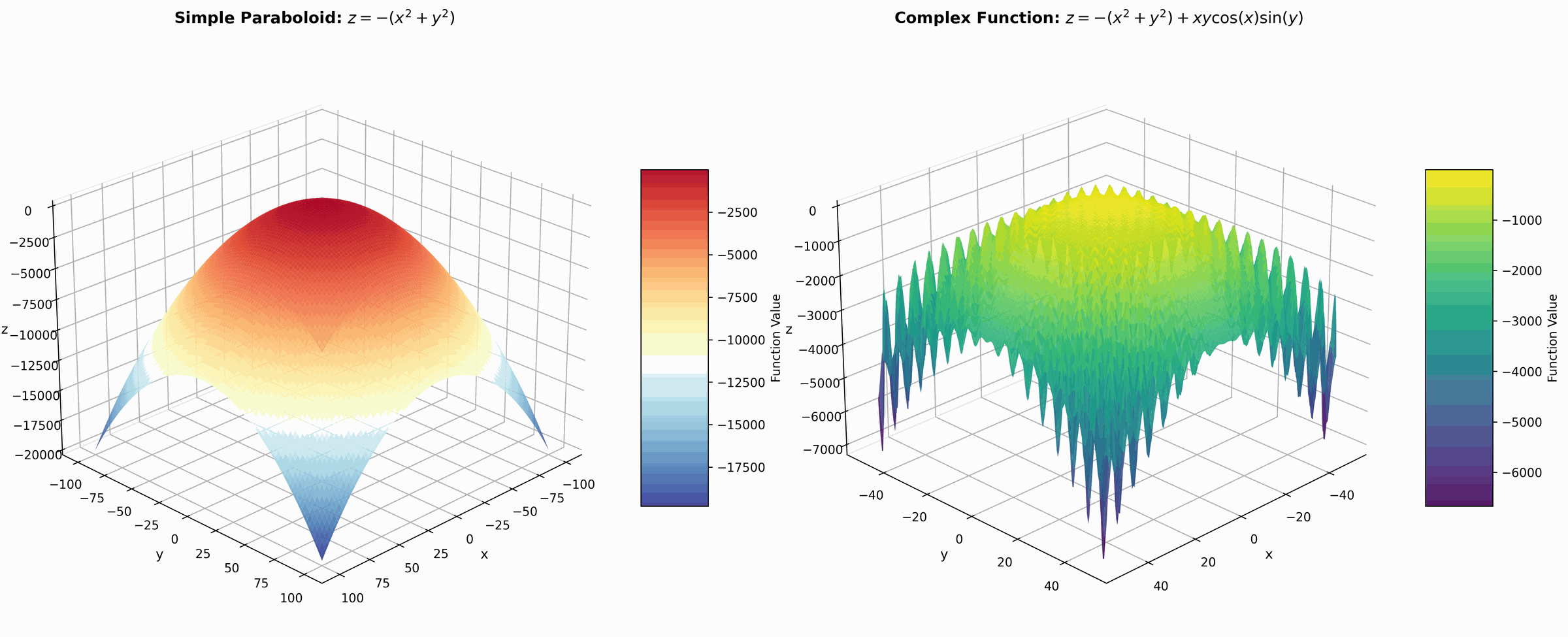
For this problem, we are going to solve an intuitive problem: function maximization. Given a function (z = f(x, y)), for what values of (x, y) will (z) be the largest? To start, we are going to use a trivial function to maximize:

$$ z = -x^2 - y^2 $$

We see it is nothing more than a paraboloid. Furthermore, since it is infinite, we are going to restrict the domain to ({ x, y \in \mathbb{Z}^+ : -100 \leq x, y \leq 100 }); therefore, we only have integer values between ((-100, 100)).

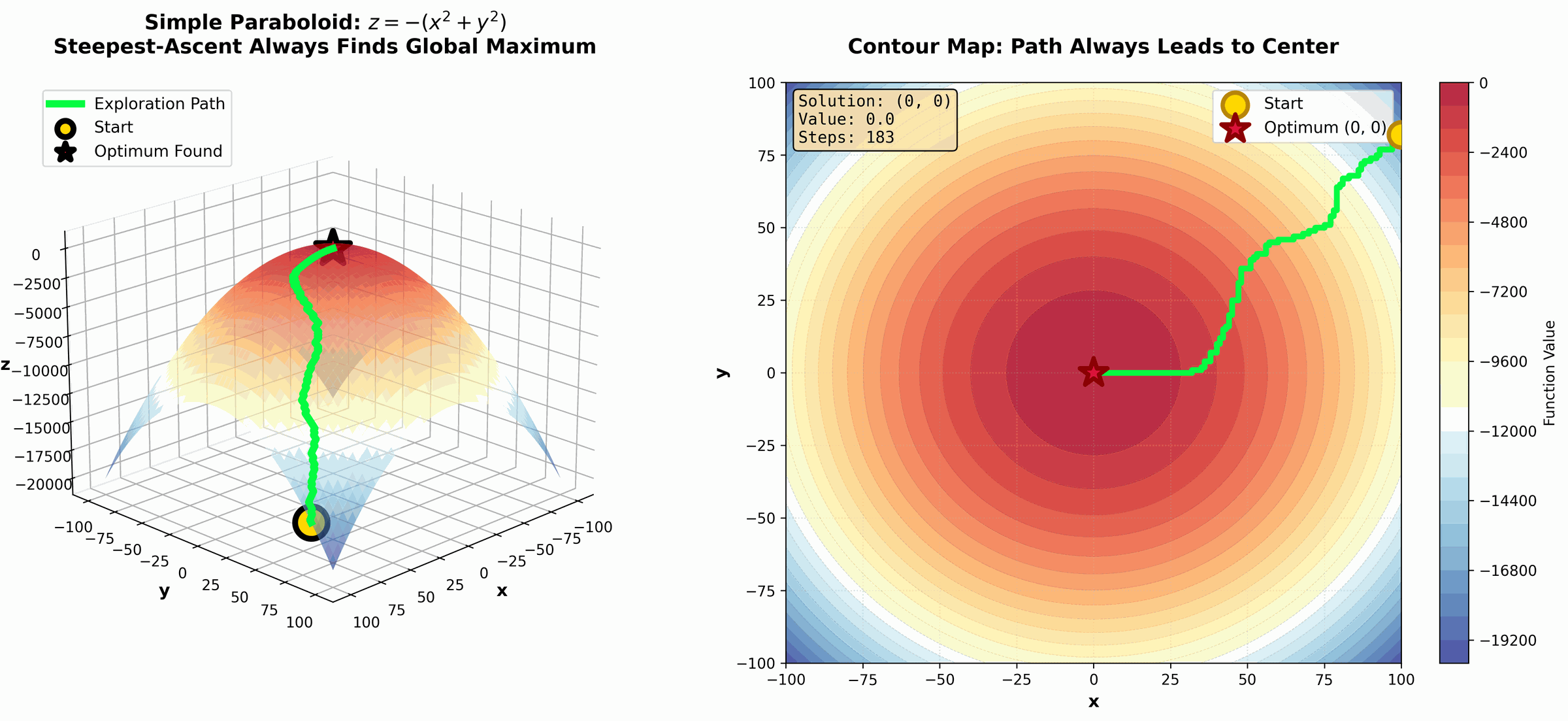
So, let's begin.

The Representation

Because we will be searching throughout a search space, we will need some representation of a state. For our particular problem instance, it's very easy: the points ((x, y)). Also, we will need to represent the (f) value, so we create an auxiliary class as well.

class Node:
    """A node in a search space (similar to a point (x, y)."""

    def __init__(self, x, y):
        self.x = x
        self.y = y


class Function:
    """A function and its respective bounds."""

    def __init__(self, function, x_bounds, y_bounds):
        ...

    def __call__(self, node):
        ...

    @property
    def x_bounds(self):
        """Get the x bounds of the function.

        Returns:
            tuple<int, int>: The x bounds of function in the format (min, max).
        """
        ...

    @property
    def y_bounds(self):
        """Get the y bounds of the function.

        Returns:
            tuple<int, int>: The y bounds of function in the format (min, max).
        """
        ...

That will be all that we need for our purposes.

Steepest-Ascent Hill-Climbing

As we saw before, there are only four moving pieces that our hill-climbing algorithm has: a way of determining the value at a node, an initial node generator, a neighbor generator, and a way of determining the highest valued neighbor.

Starting with the way of determining the value at a node, it's very intuitive: calculate the value (z = f(x, y)).

class HillClimber:
    """A steepest-ascent hill-climbing algorithm."""

    def __init__(self, function):
        self.function = function

    def _value_at_node(self, node):
        return self.function(node)

The initial node can simply be taken as a random ((x, y)) in their respective bounds.

    def _initial_node(self):
        x = randint(self.function.x_bounds[0], self.function.x_bounds[1])
        y = randint(self.function.y_bounds[0], self.function.y_bounds[1])

        return Node(x, y)

Generating neighbors is actually quite simple as well: because our domain is limited to integers, we can simply look at the four cardinal directions (and make sure we won't be breaking the bounds when we do). Also, we randomize the neighbors, to make things more interesting[^2].

    def _generate_all_neighbors(self, node):
        x, y = node.x, node.y

        nodes = [Node(x, y)]

        if x < self.function.x_bounds[1]:
            nodes.append(Node(x + 1, y))
        if x > self.function.x_bounds[0]:
            nodes.append(Node(x - 1, y))
        if y < self.function.y_bounds[1]:
            nodes.append(Node(x, y + 1))
        if y > self.function.y_bounds[0]:
            nodes.append(Node(x, y - 1))

        shuffle(nodes)
        return nodes

Finally, to get the highest value node, it's fairly straightforward:

    def _highest_valued_node(self, neighbors):
        max_point = neighbors[0]

        for point in neighbors[1:]:
            if self._value_at_node(point) > self._value_at_node(max_point):
                max_point = point

        return max_point

Piecing all this together, we get our Steepest-Ascent Hill-Climber:

  def climb(self):
        current_node = self._initial_node()

        while True:
            print("Exploring Node({}, {})".format(current_node.x,
                                                   current_node.y))
            neighbors = self._generate_all_neighbors(current_node)
            successor = self._highest_valued_node(neighbors)

            if (self._value_at_node(successor) <=
                    self._value_at_node(current_node)):
                return current_node

            current_node = successor

Does it work? Exactly as planned.

Exploring Node(5, -88)
...
Exploring Node(5, -67)
...
Exploring Node(5, -47)
...
Exploring Node(5, -27)
...
Exploring Node(5, -4)
Exploring Node(4, -4)
Exploring Node(3, -4)
Exploring Node(3, -3)
Exploring Node(2, -3)
Exploring Node(2, -2)
Exploring Node(1, -2)
Exploring Node(1, -1)
Exploring Node(1, 0)
Exploring Node(0, 0)

However, this was too easy. We had a function with one local optimum. Let's make things interesting.

Optimizing Steepest-Ascent Hill-Climbing

Suppose we keep our previous domain, but we change our function to the following:

$$ z = -(x^2 + y^2) + x\, y\, \cos x \sin y $$

This function isn't quite as intuitive to visualize, please reference the figure. Essentially, it's what we had before, but thousands of local optimum when we get further from the center. Our previous Hill-Climbing would absolutely get destroyed by that function.

Complex Hill Climbing Function with Multiple Local Optima

To alleviate this, we are going to use two optimizations:

Instead of taking the steepest uphill move, we are going to simply take a random, uphill move (known as Stochastic Hill-Climbing).
When we get stuck, we are going to restart the search (known as Hill-Climbing With Restarts).

Stochastic Hill-Climbing

Updating the algorithm is fairly simply, all the previous mechanics are inheritable, just swap out _highest_valued_node with a stochastic version.

class StochasticHillClimber(HillClimber):
    """A stochastic steepest-ascent hill-climbing algorithm."""

    def _get_random_uphill_move(self, current_node, neighbors):
        uphill_nodes = []

        for point in neighbors:
            if self._value_at_node(point) > self._value_at_node(current_node):
                uphill_nodes.append(point)

        return current_node if len(uphill_nodes) == 0 else choice(uphill_nodes)

    def climb(self):
        current_node = self._initial_node()

        while True:
            print("Exploring Node({}, {})".format(current_node.x,
                                                   current_node.y))

            neighbors = self._generate_all_neighbors(current_node)
            successor = self._get_random_uphill_move(current_node,
                                                      neighbors)

            if (self._value_at_node(successor) <=
                    self._value_at_node(current_node)):
                return current_node

            current_node = successor

Running this algorithm, we get better results; but we can do better.

Stochastic Hill-Climbing With Restarts

For this, we simply have to restructure the climb function to handle generational effects (like keeping the max valued node throughout generations). Not too difficult.

class StochasticHillClimberWithRestarts(StochasticHillClimber):
    """A stochastic steepest-ascent hill-climbing algorithm with restarts."""

    def climb(self, number_of_generations):
        max_node = self._initial_node()

        for generations in range(number_of_generations):
            current_node = self._initial_node()

            while True:
                msg = "Generation {}, Exploring Node({}, {}), " + \
                      "Current Max Node({}, {})"
                print(msg.format(generations, current_node.x,
                                 current_node.y,
                                 max_node.x, max_node.y))

                neighbors = self._generate_all_neighbors(current_node)
                successor = self._get_random_uphill_move(current_node,
                                                          neighbors)

                if (self._value_at_node(max_node) <
                        self._value_at_node(current_node)):
                    max_node = current_node

                if (self._value_at_node(successor) <=
                        self._value_at_node(current_node)):
                    break

                current_node = successor

        return max_node

How did this one fare? Quite better than all the rest. Let's take a look at what the exploration process looked like.

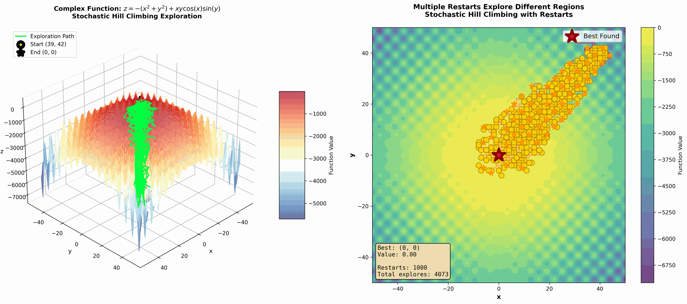
Marvelous, some got to the top, many got caught in local optimum. A global-optimum was found. A success.

[^1]: Algorithms used in games, where a player searches for an optimal move against an opponent. [^2]: If the neighbors are always generated deterministically, there might occur a sequence of ties when generating the highest-valued node. We randomize the neighbors so a random piece will be chosen in the tie-breaker.

Friday, 2 November 2018

, & Illya Starikov

AI Code Computer Science