Application
Small software that does one thing and then gets out of your way. Browser tools and toys, with no accounts and no ulterior motives.
Sorting Algorithms
sort<Algorithm>(from: bubble, to: Tim)
When I was a Teacher Assistant (TA) in Intro To Computer Science lab, fellow TA
Ian and I were showing off our programming prowess. I thought I had it in the bag: I had solved a competitive programming problem in compile-time (C++ templates are Turing-complete!) and a Space Invaders clone for a class.
But Ian was more clever than I, and showed me something that fundamentally changed how I saw a core-component of programming: a terminal-based (ncurses) sorting algorithm visualizers.
It was the first time I had ever seen these algorithms graphed like this — ever! And, yes, I blame my Algorithm instructor. I finally could see all the hypothetical sorting in a real-life application.
With the power of LLMs in hand, and a website as my canvas, I wanted to see if I could recreate this. Kudos to you, Ian.
Sorting algorithms form the backbone of computer science, serving as fundamental building blocks for countless applications from database management to search engines. This comprehensive guide examines the 25 most important sorting algorithms, organized by type, with detailed analysis of their performance, implementation, and practical applications.
1. Basic Comparison-Based Algorithms
These fundamental algorithms serve as the foundation for understanding sorting concepts, though they generally have O(n²) time complexity.
1.1 Bubble Sort
Complexity Analysis:
- Best Case: O(n) / Ω(n) - when array is already sorted
- Average Case: O(n²) / Θ(n²)
- Worst Case: O(n²)
- Space: O(1)
Properties: Stable, In-place, Adaptive
def bubble_sort(arr):
    """
    Bubble Sort with optimization
    Time: O(n²) average/worst, O(n) best
    Space: O(1)
    """
    n = len(arr)

    for i in range(n):
        swapped = False

        # Last i elements are already sorted
        for j in range(0, n - i - 1):
            if arr[j] > arr[j + 1]:
                arr[j], arr[j + 1] = arr[j + 1], arr[j]
                swapped = True

        # If no swapping occurred, array is sorted
        if not swapped:
            break

    return arr
When to Use:
- Small datasets (< 50 elements)
- Educational purposes - excellent for teaching
- Nearly sorted data
- Memory-constrained environments
Step-by-Step Example:
Array: [64, 34, 25, 12, 22, 11, 90]
Pass 1: [34, 25, 12, 22, 11, 64, 90] - Largest element "bubbles" to end
Pass 2: [25, 12, 22, 11, 34, 64, 90]
... continues until sorted
History: First described by Edward Harry Friend in 1956. The name "bubble sort" was coined by Kenneth E. Iverson due to how smaller elements "bubble" to the top.
Notable Trivia: Donald Knuth famously stated "bubble sort seems to have nothing to recommend it, except a catchy name." Despite criticism, it remains the most taught sorting algorithm due to its simplicity.
1.2 Selection Sort
Complexity Analysis:
- Best/Average/Worst Case: O(n²) - always makes same comparisons
- Space: O(1)
Properties: Unstable, In-place, Not adaptive
def selection_sort(arr):
    """
    Selection Sort implementation
    Time: O(n²) for all cases
    Space: O(1)
    """
    n = len(arr)

    for i in range(n):
        # Find minimum element in remaining unsorted array
        min_idx = i

        for j in range(i + 1, n):
            if arr[j] < arr[min_idx]:
                min_idx = j

        # Swap the found minimum element
        arr[i], arr[min_idx] = arr[min_idx], arr[i]

    return arr
When to Use:
- When memory write operations are expensive (e.g., flash memory)
- Small datasets where simplicity matters
- When the number of swaps needs to be minimized
Key Advantage: Performs only O(n) swaps compared to O(n²) for bubble sort.
History: Has ancient origins in manual sorting processes. Formalized in the 1950s as one of the fundamental sorting methods.
1.3 Insertion Sort
Complexity Analysis:
- Best Case: O(n) - already sorted
- Average/Worst Case: O(n²)
- Space: O(1)
Properties: Stable, In-place, Adaptive, Online
def insertion_sort(arr):
    """
    Insertion Sort implementation
    Time: O(n²) average/worst, O(n) best
    Space: O(1)
    """
    for i in range(1, len(arr)):
        key = arr[i]
        j = i - 1

        while j >= 0 and arr[j] > key:
            arr[j + 1] = arr[j]
            j -= 1

        arr[j + 1] = key

    return arr
When to Use:
- Small datasets (typically < 50 elements)
- Nearly sorted data - performs in O(n) time
- Online algorithms - when data arrives sequentially
- As a subroutine in quicksort and mergesort for small subarrays
Notable Use: Used in Timsort (Python's built-in sort) for small runs. Often faster than O(n log n) algorithms for arrays with fewer than 10-20 elements.
1.4 Shell Sort
Complexity Analysis:
- Best Case: O(n log n)
- Average Case: O(n^1.25) to O(n^1.5) depending on gap sequence
- Worst Case: O(n²) for Shell's original sequence
- Space: O(1)
Properties: Unstable, In-place, Adaptive
def shell_sort(arr):
    """
    Shell Sort using Shell's original sequence
    Time: O(n²) worst case, O(n log n) average
    Space: O(1)
    """
    n = len(arr)
    gap = n // 2

    while gap > 0:
        # Perform gapped insertion sort
        for i in range(gap, n):
            temp = arr[i]
            j = i

            while j >= gap and arr[j - gap] > temp:
                arr[j] = arr[j - gap]
                j -= gap

            arr[j] = temp

        gap //= 2

    return arr
When to Use:
- Medium-sized datasets (100-5000 elements)
- When recursion should be avoided
- Embedded systems - simple and efficient
History: Invented by Donald L. Shell in 1959, it was one of the first algorithms to break the O(n²) barrier.
1.5 Cocktail Shaker Sort (Bidirectional Bubble Sort)
Complexity Analysis:
- Best Case: O(n)
- Average/Worst Case: O(n²)
- Space: O(1)
Properties: Stable, In-place, Adaptive, Bidirectional
def cocktail_shaker_sort(arr):
    """
    Cocktail Shaker Sort (Bidirectional Bubble Sort)
    Time: O(n²) average/worst, O(n) best
    Space: O(1)
    """
    n = len(arr)
    start = 0
    end = n - 1

    while start < end:
        swapped = False

        # Forward pass
        for i in range(start, end):
            if arr[i] > arr[i + 1]:
                arr[i], arr[i + 1] = arr[i + 1], arr[i]
                swapped = True

        if not swapped:
            break

        end -= 1
        swapped = False

        # Backward pass
        for i in range(end, start, -1):
            if arr[i] < arr[i - 1]:
                arr[i], arr[i - 1] = arr[i - 1], arr[i]
                swapped = True

        if not swapped:
            break

        start += 1

    return arr
Advantage: Better than bubble sort at moving small elements (turtles) to the beginning.
2. Efficient Comparison-Based Algorithms
These algorithms achieve O(n log n) average performance and form the backbone of many practical sorting implementations.
2.1 Quick Sort
Complexity Analysis:
- Best/Average Case: O(n log n)
- Worst Case: O(n²) - when pivot is always minimum/maximum
- Space: O(log n) - recursion stack
Properties: Unstable, In-place, Not adaptive
def quicksort(arr, low=0, high=None):
    """
    Quicksort with Hoare partition scheme
    Time: O(n log n) average, O(n²) worst
    Space: O(log n)
    """
    if high is None:
        high = len(arr) - 1

    if low < high:
        pivot_idx = partition(arr, low, high)
        quicksort(arr, low, pivot_idx)
        quicksort(arr, pivot_idx + 1, high)

    return arr

def partition(arr, low, high):
    """Hoare partition scheme"""
    pivot = arr[low]
    i = low - 1
    j = high + 1

    while True:
        i += 1
        while arr[i] < pivot:
            i += 1

        j -= 1
        while arr[j] > pivot:
            j -= 1

        if i >= j:
            return j

        arr[i], arr[j] = arr[j], arr[i]
Why It's Preferred Despite O(n²) Worst Case:
- Excellent average-case performance with good constant factors
- Cache-friendly sequential access patterns
- In-place sorting
- Modern implementations use introsort to guarantee O(n log n)
History: Invented by Tony Hoare in 1959 while working on machine translation at Moscow State University.
2.2 Merge Sort
Complexity Analysis:
- All Cases: O(n log n) - guaranteed performance
- Space: O(n) - requires additional space for merging
Properties: Stable, Not in-place, Not adaptive
def merge_sort(arr):
    """
    Merge Sort implementation
    Time: O(n log n) guaranteed
    Space: O(n)
    """
    if len(arr) <= 1:
        return arr

    mid = len(arr) // 2
    left = merge_sort(arr[:mid])
    right = merge_sort(arr[mid:])

    return merge(left, right)

def merge(left, right):
    """Merge two sorted arrays"""
    result = []
    i = j = 0

    while i < len(left) and j < len(right):
        if left[i] <= right[j]:
            result.append(left[i])
            i += 1
        else:
            result.append(right[j])
            j += 1

    result.extend(left[i:])
    result.extend(right[j:])

    return result
When to Use:
- When stability is required
- External sorting (large datasets that don't fit in memory)
- Linked lists (efficient with O(1) extra space)
- Parallel processing
History: Invented by John von Neumann in 1945, with detailed analysis published in 1948.
2.3 Heap Sort
Complexity Analysis:
- All Cases: O(n log n) - guaranteed performance
- Space: O(1) - true in-place sorting
Properties: Unstable, In-place, Not adaptive
def heap_sort(arr):
    """
    Heap Sort implementation
    Time: O(n log n) guaranteed
    Space: O(1)
    """
    n = len(arr)

    # Build max heap
    for i in range(n // 2 - 1, -1, -1):
        heapify(arr, n, i)

    # Extract elements from heap
    for i in range(n - 1, 0, -1):
        arr[0], arr[i] = arr[i], arr[0]
        heapify(arr, i, 0)

    return arr

def heapify(arr, n, i):
    """Maintain heap property"""
    largest = i
    left = 2 * i + 1
    right = 2 * i + 2

    if left < n and arr[left] > arr[largest]:
        largest = left

    if right < n and arr[right] > arr[largest]:
        largest = right

    if largest != i:
        arr[i], arr[largest] = arr[largest], arr[i]
        heapify(arr, n, largest)
When to Use:
- Memory-constrained environments
- Real-time systems (guaranteed performance)
- Systems concerned with malicious input
History: Invented by J. W. J. Williams in 1964, with in-place version by Robert Floyd.
2.4 Binary Tree Sort
Complexity Analysis:
- Best/Average Case: O(n log n) - with balanced tree
- Worst Case: O(n²) - with unbalanced tree
- Space: O(n) - for tree structure
Properties: Can be stable, Not in-place
When to Use:
- Educational purposes
- When tree structure is needed for other operations
- Online sorting
Note: Self-balancing trees (AVL, Red-Black) guarantee O(n log n) performance.
2.5 Smooth Sort
Complexity Analysis:
- Best Case: O(n) - for sorted data
- Average/Worst Case: O(n log n)
- Space: O(1)
Properties: Unstable, In-place, Adaptive
History: Invented by Edsger W. Dijkstra in 1981 as an improvement over heapsort for partially sorted data.
Notable Use: Used in musl C library's qsort() implementation.
3. Non-Comparison Based Algorithms
These algorithms achieve linear O(n) time complexity by exploiting specific properties of the data rather than comparing elements.
3.1 Counting Sort
Complexity Analysis:
- All Cases: O(n + k) where k is the range of values
- Space: O(n + k)
Properties: Stable, Not in-place
def counting_sort(arr):
    """
    Counting Sort for non-negative integers
    Time: O(n + k)
    Space: O(n + k)
    """
    if not arr:
        return arr

    max_val = max(arr)
    count = [0] * (max_val + 1)

    # Count occurrences
    for num in arr:
        count[num] += 1

    # Calculate cumulative count
    for i in range(1, len(count)):
        count[i] += count[i - 1]

    # Build output array
    output = [0] * len(arr)
    for i in range(len(arr) - 1, -1, -1):
        output[count[arr[i]] - 1] = arr[i]
        count[arr[i]] -= 1

    return output
When to Use:
- Sorting integers in a small range
- As a subroutine in radix sort
- When k is O(n) or smaller
History: Invented by Harold H. Seward in 1954 at MIT.
3.2 Radix Sort
Complexity Analysis:
- All Cases: O(d × (n + k)) where d is number of digits
- Space: O(n + k)
Properties:
- LSD (Least Significant Digit): Stable
- MSD (Most Significant Digit): Can be stable
def radix_sort_lsd(arr):
    """
    LSD Radix Sort implementation
    Time: O(d × (n + k))
    Space: O(n + k)
    """
    if not arr:
        return arr

    max_val = max(arr)
    exp = 1

    while max_val // exp > 0:
        counting_sort_for_radix(arr, exp)
        exp *= 10

    return arr

def counting_sort_for_radix(arr, exp):
    n = len(arr)
    output = [0] * n
    count = [0] * 10

    for i in range(n):
        index = arr[i] // exp
        count[index % 10] += 1

    for i in range(1, 10):
        count[i] += count[i - 1]

    i = n - 1
    while i >= 0:
        index = arr[i] // exp
        output[count[index % 10] - 1] = arr[i]
        count[index % 10] -= 1
        i -= 1

    for i in range(n):
        arr[i] = output[i]
When to Use:
- Sorting integers with many digits
- String sorting (MSD variant)
- When d is small compared to log n
History: Dates back to 1887 with Herman Hollerith's tabulating machines.
3.3 Bucket Sort
Complexity Analysis:
- Best/Average Case: O(n + k) for uniform distribution
- Worst Case: O(n²) when all elements fall into one bucket
- Space: O(n + k)
Properties: Stable (if sub-sorting is stable), Not in-place
def bucket_sort(arr):
    """
    Bucket Sort for floating-point number
    Time: O(n + k) average
    Space: O(n + k)
    """
    if not arr:
        return arr

    min_val, max_val = min(arr), max(arr)
    bucket_count = len(arr)
    buckets = [[] for _ in range(bucket_count)]

    # Distribute elements into buckets
    for num in arr:
        if max_val == min_val:
            index = 0
        else:
            index = int((num - min_val) / (max_val - min_val) * (bucket_count - 1))
        buckets[index].append(num)

    # Sort individual buckets
    result = []
    for bucket in buckets:
        if bucket:
            bucket.sort()  # Can use insertion sort
            result.extend(bucket)

    return result
When to Use:
- Uniformly distributed floating-point numbers
- Large datasets with known range
- When memory is not a constraint
3.4 Pigeonhole Sort
Complexity Analysis:
- All Cases: O(n + range) where range = max - min + 1
- Space: O(range)
Properties: Stable, Not in-place
When to Use:
- Small range of integer values
- When range is comparable to n
- Simple counting applications
History: Based on the pigeonhole principle, formally described by A.J. Lotka (1926).
3.5 Flash Sort
Complexity Analysis:
- Best/Average Case: O(n) for uniform distribution
- Worst Case: O(n²)
- Space: O(m) where m is number of classes
Properties: Unstable, In-place (major advantage)
When to Use:
- Large uniformly distributed datasets
- When memory is limited
- When O(n) average performance is critical
History: Invented by Karl-Dietrich Neubert in 1998 as an efficient in-place implementation of bucket sort.
4. Modern Hybrid Algorithms
These algorithms represent the state-of-the-art in practical sorting, combining multiple techniques for superior performance.
4.1 Timsort
Complexity Analysis:
- Best Case: O(n) - already sorted
- Average/Worst Case: O(n log n)
- Space: O(n)
Properties: Stable, Not in-place
Key Innovations:
- Run Detection: Identifies naturally occurring sorted subsequences
- Minimum Run Size: Calculates optimal minrun (32-64 elements)
- Galloping Mode: Switches to exponential search when one run consistently "wins"
Where It's Used:
- Python's default sort since version 2.3
- Java for sorting objects (Java 7+)
- Android, V8, Swift, Rust
History: Created in 2002 by Tim Peters for Python. A critical bug was discovered and fixed in 2015 through formal verification.
4.2 Introsort (Introspective Sort)
Complexity Analysis:
- All Cases: O(n log n) - guaranteed by heapsort fallback
- Space: O(log n)
Properties: Unstable, In-place
Techniques Combined:
- Quicksort for main sorting
- Heapsort when recursion depth exceeds 2×log₂(n)
- Insertion sort for small subarrays (< 16 elements)
Where It's Used:
- C++ STL's std::sort() in GCC and LLVM
- Microsoft .NET Framework 4.5+
History: Created by David Musser in 1997 to provide guaranteed O(n log n) performance while maintaining quicksort's average-case speed.
4.3 Block Sort (WikiSort)
Complexity Analysis:
- Best Case: O(n)
- Average/Worst Case: O(n log n)
- Space: O(1) - constant space!
Properties: Stable, In-place
Key Innovation: Achieves stable merge sort performance with O(1) space by using internal buffering.
When to Use: When O(1) space complexity and stability are both required.
4.4 Pattern-defeating Quicksort (pdqsort)
Complexity Analysis:
- Best Case: O(n) for specific patterns
- Average/Worst Case: O(n log n)
- Space: O(log n)
Properties: Unstable, In-place
Key Innovations:
- Pattern detection and optimization
- Branchless partitioning
- Adaptive strategy based on input characteristics
Where It's Used:
- Rust's default unstable sort
- C++ Boost libraries
History: Created by Orson Peters in 2016 to improve upon introsort with better pattern handling.
4.5 Dual-Pivot Quicksort
Complexity Analysis:
- Best Case: O(n) when all elements equal
- Average Case: O(n log n) - 5% fewer comparisons than single-pivot
- Worst Case: O(n²) - still possible but less likely
- Space: O(log n)
Properties: Unstable, In-place
Key Innovation: Uses two pivots to partition array into three parts, reducing comparisons.
Where It's Used: Java's default algorithm for primitive arrays since Java 7.
History: Created by Vladimir Yaroslavskiy in 2009, adopted by Java in 2011.
5. Specialized and Educational Algorithms
These algorithms serve specific purposes or demonstrate important concepts in computer science education.
5.1 Comb Sort
Complexity Analysis:
- Best Case: O(n log n)
- Average Case: O(n²/2^p) where p is number of increments
- Worst Case: O(n²)
- Space: O(1)
Properties: Unstable, In-place
Key Feature: Improves upon bubble sort using variable gap with shrink factor of 1.3.
History: Developed by Włodzimierz Dobosiewicz in 1980 to address bubble sort's inefficiency.
5.2 Gnome Sort (Stupid Sort)
Complexity Analysis:
- Best Case: O(n)
- Average/Worst Case: O(n²)
- Space: O(1)
Properties: Stable, In-place, Adaptive
Unique Feature: Uses only a single while loop - inspired by garden gnomes sorting flower pots.
5.3 Cycle Sort
Complexity Analysis:
- All Cases: O(n²)
- Space: O(1)
Properties: Unstable, In-place
Key Feature: Minimizes memory writes - each element is written at most once to its correct position.
When to Use: When memory write operations are expensive (EEPROM, Flash memory).
5.4 Pancake Sort
Complexity Analysis:
- Best Case: O(n)
- Average/Worst Case: O(n²)
- Space: O(1)
Properties: Unstable, In-place
Unique Constraint: Only allowed operation is "flip" (reverse prefix).
Historical Note: Bill Gates' only published academic paper was on this problem (1979), providing a (5n+5)/3 upper bound algorithm.
5.5 Bogo Sort
Complexity Analysis:
- Best Case: O(n) - already sorted
- Average Case: O(n·n!) - expected permutations
- Worst Case: O(∞) - theoretically unbounded
- Space: O(1)
Properties: Unstable, In-place
Educational Value:
- Demonstrates worst-case analysis
- Teaches randomized algorithms
- Shows importance of algorithm selection
import random

def bogo_sort(arr):
    """The worst sorting algorithm ever conceived"""
    def is_sorted(arr):
        return all(arr[i] <= arr[i+1] for i in range(len(arr)-1))

    while not is_sorted(arr):
        random.shuffle(arr)

    return arr
Trivia: "Quantum Bogo Sort" hypothetically destroys universes where array isn't sorted, leaving only sorted universes.
Summary and Recommendations
Performance Comparison Table
| Algorithm | Best Case | Average Case | Worst Case | Space | Stable | In-Place |
|---|---|---|---|---|---|---|
| Bubble Sort | O(n) | O(n²) | O(n²) | O(1) | Yes | Yes |
| Selection Sort | O(n²) | O(n²) | O(n²) | O(1) | No | Yes |
| Insertion Sort | O(n) | O(n²) | O(n²) | O(1) | Yes | Yes |
| Quick Sort | O(n log n) | O(n log n) | O(n²) | O(log n) | No | Yes |
| Merge Sort | O(n log n) | O(n log n) | O(n log n) | O(n) | Yes | No |
| Heap Sort | O(n log n) | O(n log n) | O(n log n) | O(1) | No | Yes |
| Counting Sort | O(n+k) | O(n+k) | O(n+k) | O(n+k) | Yes | No |
| Radix Sort | O(d(n+k)) | O(d(n+k)) | O(d(n+k)) | O(n+k) | Yes | No |
| Timsort | O(n) | O(n log n) | O(n log n) | O(n) | Yes | No |
When to Use Which Algorithm
For Small Datasets (< 50 elements):
- Insertion Sort - simple and efficient
- Selection Sort - when minimizing swaps matters
For General Purpose:
- Timsort (Python) or Introsort (C++) - best overall performance
- Quick Sort with good pivot selection - excellent average case
For Guaranteed Performance:
- Merge Sort - stable and predictable
- Heap Sort - when O(1) space is required
For Special Data Types:
- Counting Sort - small integer ranges
- Radix Sort - large integers or strings
- Bucket Sort - uniformly distributed floats
For Educational Purposes:
- Start with Bubble Sort for simplicity
- Progress to Quick Sort and Merge Sort
- Use Bogo Sort to demonstrate algorithm analysis
Key Takeaways
- No single best algorithm - choice depends on data characteristics, constraints, and requirements
- Modern algorithms are hybrids - combining techniques yields superior performance
- Stability matters for sorting complex objects where maintaining relative order is important
- Space-time tradeoffs are crucial - some algorithms trade memory for speed
- Real-world performance often differs from theoretical complexity due to cache effects, data patterns, and implementation details
Understanding these 25 algorithms provides a comprehensive foundation for tackling sorting problems in any context, from embedded systems to large-scale data processing.

Dice
Roll With It

Home Row
112 WPM. Take that, typing teacher!
I managed a new high score in TypeRacer today: 112WPM.
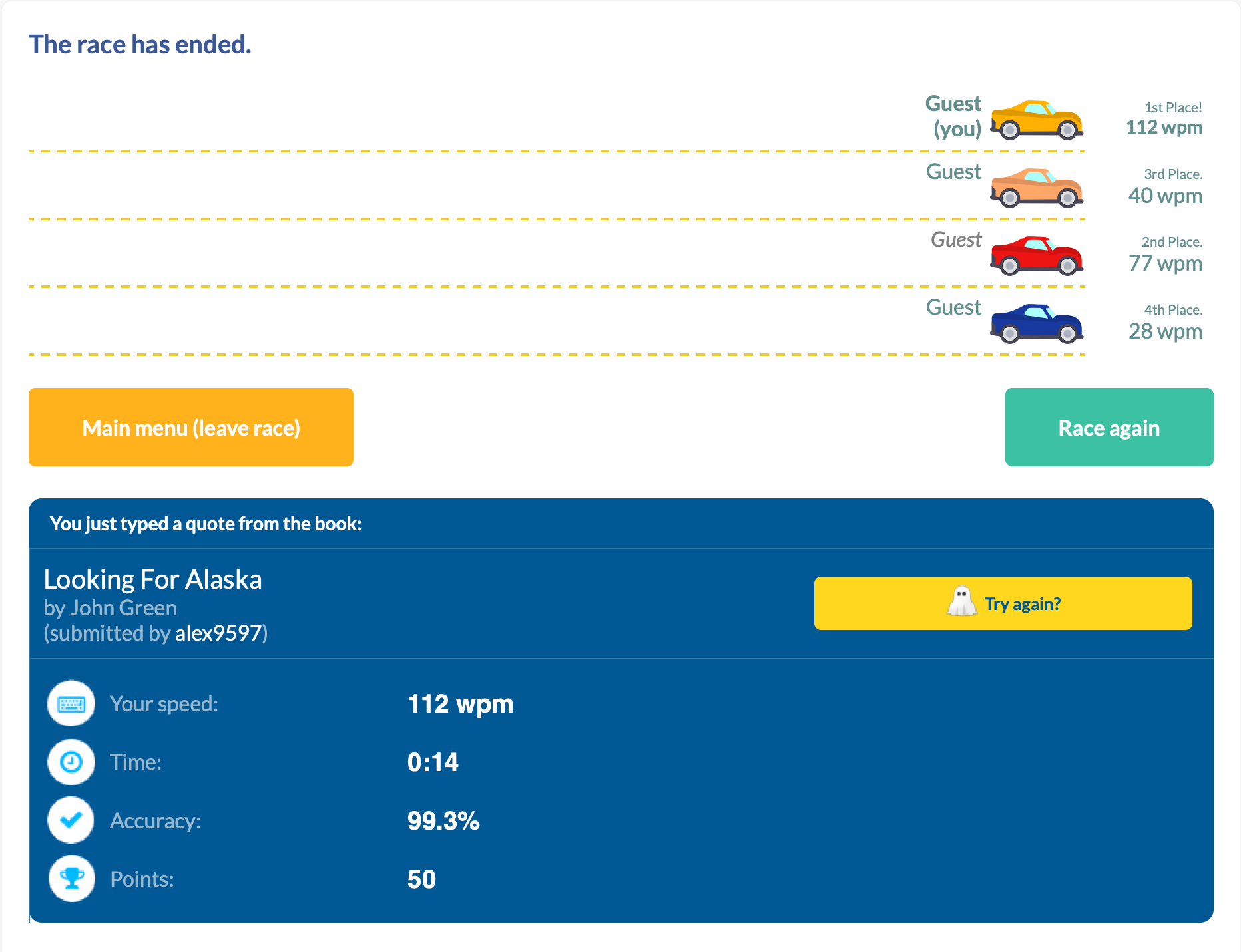
With this article, I wanted to share my journey here, and how I would recommend someone to start.
My Typing Story
I have an interesting history with typing.
I started "typing" at age of five years old to learn the controls of Quake. While the keyboard was a different language with different characters, the muscle memory was the same keyboard-to-keyboard. Upon moving to the states, I changed to an English QWERTY keyboard, and continued playing Doom.
In middle school, before beginning typing class, I clocked in at 35-40 WPM. As I progressed throughout the class, I got familiar with more of the "weird" keys (symbols, numbers, q/z/v) and what a proper "home-row" hand positioning looked like. Midway through the class, I made a discovery about our typing software: you were allowed to make two mistakes, with one word misspell counting as one mistake, and at the end the software took the number of characters you had finished and divided it by 5 (the average word length). So I typed a few words, then held down a random key until the timer expired. And scored 230 WPM.
I thought I was going to get credit for finding a bug our school's software; while my teacher did call my parents that night, it was accuse me of hacking the typing software and changing my score. After explaining to her what I did, her first remedy suggested was a generous failing grade and suspension, but after apologizing to her and the staff, I was only forbidden from being crowned best typist at the school assembly. I may have not gotten an award, but I kept typing skills, reaching 55-65 WPM consistently.
In high school, it was more of the same classes, so I didn't see my typing speed increase drastically—I hovered in the 60-70 WPM range. Even in college, I plateaued around this range.
That is, until I got a mechanical keyboard. I didn't see the results immediately, but with consistent use I bumped my numbers to 65-80 WPM. And this is where I hovered for 5 years; this is where I felt like I had maxed out given the same environment.
I couldn't get any better, because my hand movement prohibited it. While my core fingers mostly stayed in home-row, to achieve my top speed I had developed bad habits to maintain it. Habits such as using right (dominant) index finger to go 3 keys over to the left or using my ring finger in-place of my little finger. While I always returned to home-row, I could feel the excess movement taking its toll, both on my efficiency and general hand strain. During the pandemic, I was working on my computer a lot, and my hands just could not keep up.
So for the first time since I started typing I had to try. It's hard to rewire muscle memory, especially at 30. I tried perfecting every keystroke, getting a massive dopamine hit as I consistently landed the ones I use most often. However, that last 20% feels much harder than the first 20%.
Today, I still try to perfect my craft. I still struggle with my little finger movement. I still catch myself trying to regress some of my old ways when I am trying to compensate and type fast. But today I also typed 112 WPM, and that's cause to celebrate. Take that, typing teacher.
You Too Can Improve
While I can't teach touch typing in a single blog post, I can give a pretty decent summary of it. The following are things I recommend doing in order to become a better typist.
Keyboard
I'll just state it outright: there's no conclusive evidence that ergonomic keyboards actually prevent RSI. Keyboards measurably improve your posture, just not necessarily your health outcomes:
- Alice layouts (Keychron V10, Epomaker Alice) reduce ulnar deviation with 10-degree inward tilt, 2-4 week learning curve
- Fully split keyboards (ErgoDox EZ, ZSA Moonlander) offer maximum adjustability including 0-60 degree tenting, 2-6 weeks to adapt
- Column-staggered designs (Corne, Kyria, Dactyl Manuform) optimize for finger lengths, brutal 1-3 month adaptation
- Kinesis Advantage2 reduces muscle activity in key flexor/extensor muscles, 2 weeks to full mastery
- Traditional ergonomic boards (Microsoft Sculpt, Logitech ERGO K860) offer gentle splits with fixed angles, ~1 month learning curve
- Alternative layouts (Dvorak, Colemak) claim reduced finger travel but have zero clinical trials and 1-3 months of productivity loss
The biomechanical improvements are real and measurable; the clinical benefits remain frustratingly theoretical.
But here's the thing: you don't need empirical evidence on the health benefits if you enjoy typing that much more. Think of it as fun with benefits (FwB, for short...). If you enjoy sitting down at your desk and typing, and it's something you do several hours a day, a keyboard you enjoy could be the push you need to improve other parts of your typing too.
Home Row
Touch typing technique centers on the home row position—ASDF for the left hand and JKL; for the right hand. The F and J keys contain tactile bumps that allow positioning without visual confirmation. This central position minimizes finger travel distance, with proper technique requiring only 0.76-1.5 key distances per character compared to 3.5+ for hunt-and-peck typing.
Each finger has specific responsibilities:
| Hand | Finger | Home Row | Keys Covered |
|---|---|---|---|
| Left | Pinky | A |
Q, A, Z, Tab, Caps Lock, Shift, ` |
| Left | Ring | S |
W, S, X, 2 |
| Left | Middle | D |
E, D, C, 3 |
| Left | Index | F |
R, F, V, T, G, B, 4, 5 |
| Right | Index | J |
Y, H, N, U, J, M, 6, 7 |
| Right | Middle | K |
I, K, ,, 8 |
| Right | Ring | L |
O, L, ., 9 |
| Right | Pinky | ; |
P, ;, /, 0, -, =, [, ], ,, ', Enter, Backspace |
| Both | Thumbs | Space |
Space only |
The index fingers cover the most keys (two columns each), while pinkies cover their column plus all outer keys. After striking any key, fingers must return to home row position—this maintains spatial orientation and prevents positional drift that increases error rates.
Ergonomics
Wrists should remain in neutral position: straight in alignment with forearms, neither bent upward (extension), downward (flexion), nor sideways. During active typing, wrists should float 1-2 inches above the keyboard surface, not resting on the desk or wrist rest. Resting creates contact stress and forces non-neutral positions. Wrist rests serve only for pauses between typing bursts.
Fingers should curve gently, similar to holding a tennis ball. This natural curve allows fingertips to strike keys perpendicularly with optimal mechanical advantage. Palms stay raised above the keyboard while hands maintain this curved posture. The biomechanics of each keystroke involve three distinct muscle activation bursts: extensor muscles lift the finger, flexor muscles drive it downward against keyswitch resistance, and extensors again remove the fingertip. Collision with the end of key travel stops downward motion, not muscle action—meaning excessive force provides no benefit and increases cumulative joint stress.
Arms should hang naturally at the sides with elbows forming 90-110 degree angles. This open angle promotes blood circulation and prevents nerve compression at the elbow. Shoulders remain relaxed and slightly externally rotated, not hunched or rolled forward.
Strength Training
Strength training shows what ergonomic keyboards can't: actual evidence. Research suggests it can significantly reduce injury risk, with clear biological reasons why—it strengthens tendons, improves tissue resilience, and builds endurance in the muscles you use for typing. The formula is simple: use weights or resistance bands (not just bodyweight), train 2-3 times weekly with rest days between, and focus on your forearms, grip, and upper back. Just be patient—tendons adapt slower than muscles, so it takes months to see results.
Conclusion
There's a learning curve to typing. In the beginning you'll see gains with minimal effort, just by knowing roughly where the keys are. As you progress and focus more on your speed, you might sacrifice hand placement (accuracy) for quickly hitting the correct key (speed). As you plateau, it will take more and more focus to correct the muscle memory. And along the way, your typing teacher may try to expel you.
All that matters is fixing your fingers, one key at a time.

Peg Solitaire
Leave The Last Peg Standing
Peg Solitaire is a classic single-player puzzle game where you jump pegs to remove them from the board, aiming to leave as few pegs as possible.
How To Play
Jump pegs over adjacent pegs to remove them from the board. Your goal is to end with as few pegs as possible - ideally just one.
Basic Rules
- Click a peg to select it (it will bounce)
- Click an empty hole to jump there
- You can only jump over one adjacent peg into an empty hole
- The jumped peg is removed
- Jumps must be horizontal or vertical (no diagonals)
- Game ends when no valid moves remain
Controls
- Click pegs - Select and move
- Undo/Redo - Take back or replay moves
- Ctrl+Z/Y - Keyboard shortcuts for undo/redo
- Theme Nine color themes: Sapphire, Ocean, Mint, Forest, Sunset, Lavender, Cherry, Slate, Honey
- Max Score - Shows the best possible outcome from current position
- Autosolve - Watch the computer find an optimal solution
- New Game - Start fresh
- Esc - Stop autosolve or close end screen
Game Modes
Board Types
- Triangular (15 holes) - Classic Cracker Barrel puzzle
- English Cross (33 holes) - Traditional European board
- French/European (37 holes) - Octagonal variant
- Diamond (41 holes) - Diamond-shaped challenge
- Wiegleb German (45 holes) - Extended cross pattern
- Asymmetrical (39 holes) - Unique irregular layout
Starting Positions
Choose where to place the initial empty hole:
- Center (most common)
- Corner (varies by board)
- Edge/Other positions
Note: Some boards have mathematically unsolvable starting positions. The game will warn you.
Achievements
Achievement tiers scale with board complexity, the fewer pegs left standing the better:
- Small Boards (15-20 holes)
1Perfect/Genius2-3Excellent4-5Good6+Keep Trying
- Medium Boards (33-37 holes)
1Perfect2-5Excellent to Very Good6-12Good to Fair13+Need Practice
- Large Boards (41-45 holes)
1-2Master3-5Expert6-14Advanced to Intermediate15+Beginner
Tips
- Plan ahead - think 2-3 moves in advance
- Try to avoid isolating pegs in corners
- Creating long chains of jumps is key to low scores
- The triangular board has over 6,000 winning sequences
- Perfect games aren't always possible from every starting position

Tea Brewing Guide
If you are cold, tea will warm you; if you are too heated, it will cool you; if you are depressed, it will cheer you; if you are excited, it will calm you.
The gap between a good cup of tea and a bitter one is usually ten degrees of water, or thirty seconds of steeping. People have been drinking tea for thousands of years and most of us still get it wrong: water straight off the boil poured over green leaves, a bag left in long enough to turn the cup to tannin. The leaf is rarely the problem. The water and the clock are.
The tool below handles the part that is just numbers. Pick a tea and it gives you the water temperature, the steeping time, how many times the leaves will keep giving, the caffeine, what it pairs with, and a timer keyed to the steep that chimes when the cup is ready. Toggle between Fahrenheit and Celsius, and, where a tea supports it, between a Western mug and gongfu's short repeated infusions. Start there.
That gets you a correct cup. The rest of this is why the numbers are what they are.
The two things that matter
Temperature and time. Everything else is refinement.
Heat is the bigger lever. Delicate leaves, white and green and yellow, scald in water near boiling: the result is bitter and flat, and no amount of sweetener brings it back. They want water that has come off the boil and rested, somewhere around 175°F. Fully oxidized leaves, black and pu-erh, and every herbal infusion, want the opposite, a hard boil to pull the flavor out at all. Oolong sits in the middle and shifts with the roast.
Time is the lever you keep your hand on. The timer starts at the short end of the recommended range on purpose. Taste it there, then extend. A cup steeped thirty seconds too long cannot be walked back; one pulled early can always go in again.
Why one leaf becomes six teas
White, yellow, green, oolong, black, and pu-erh all come from the same plant, Camellia sinensis. What separates them is oxidation, the slow browning that happens when a picked leaf meets air, the same reaction that darkens a cut apple.
White tea is the leaf barely touched, withered and dried and nothing more. Green tea is heat-fixed within hours of picking, the oxidation stopped before it starts, which is why it stays grassy and bright. Yellow is green tea given an extra sealed, slow yellowing that most producers no longer bother with, which is why you have probably never had it. Oolong is caught in the middle, anywhere from lightly to mostly oxidized, which makes it the widest category of all. Black tea is taken the whole way. Pu-erh is the outlier: not oxidized but fermented, aged for years or decades by live microbes, the only tea that genuinely improves in storage.
Six teas, one bush, one variable turned up by degrees.
Gongfu versus the mug
There are two ways to brew, and the tool will time either.
The Western way is one long steep: a teaspoon of leaf, a full mug, three to five minutes, done. It is simple, and it is most of how tea gets drunk in the world.
Gongfu is the opposite bet. A lot of leaf, a small pot, and a run of very short infusions, the first sometimes only ten seconds. You pour, drink, and pour again, and the tea changes cup to cup as the leaves open. It asks more of you, and it is the right tool for a good oolong or an aged pu-erh, which can give a dozen infusions or more before they are spent. The gongfu mode counts the steeps and adds a little time with each round, the way you would by hand.
Re-steeping, and when a leaf is done
Cheap, broken-leaf tea gives one cup and quits. Whole-leaf tea gives many, and the good ones get more interesting partway through rather than weaker. A quality oolong is often best on its third or fourth infusion; aged pu-erh can run past twenty.
Rolled and compressed teas, ball-rolled oolong and pressed pu-erh cakes, want a quick rinse first: a few seconds of hot water poured over and thrown away, which wakes the leaves and washes off storage. After that, keep going until the cup tastes thin. The leaf will tell you it is finished before any clock does.
Herbal infusions are not tea
Chamomile, rooibos, peppermint, ginger, hibiscus, lavender: none of them contain a tea leaf. They are tisanes, brewed from flowers, leaves, and roots, and the category is older than tea itself. Because there is no Camellia sinensis in the cup, they are all caffeine-free, which is most of the reason people reach for them at night.
They are also forgiving. A full boil and a long steep, five to ten minutes, will not turn them bitter the way it would a green tea, and several hold their heat and flavor long after a true tea would fade. The popular ones are in the tool above, brewed by the same two numbers as everything else.
